Appendix C. Proposed marine protected areas in the California North Central Coast Region and description of one-dimensional representation of two-dimensional coastal habitat maps.
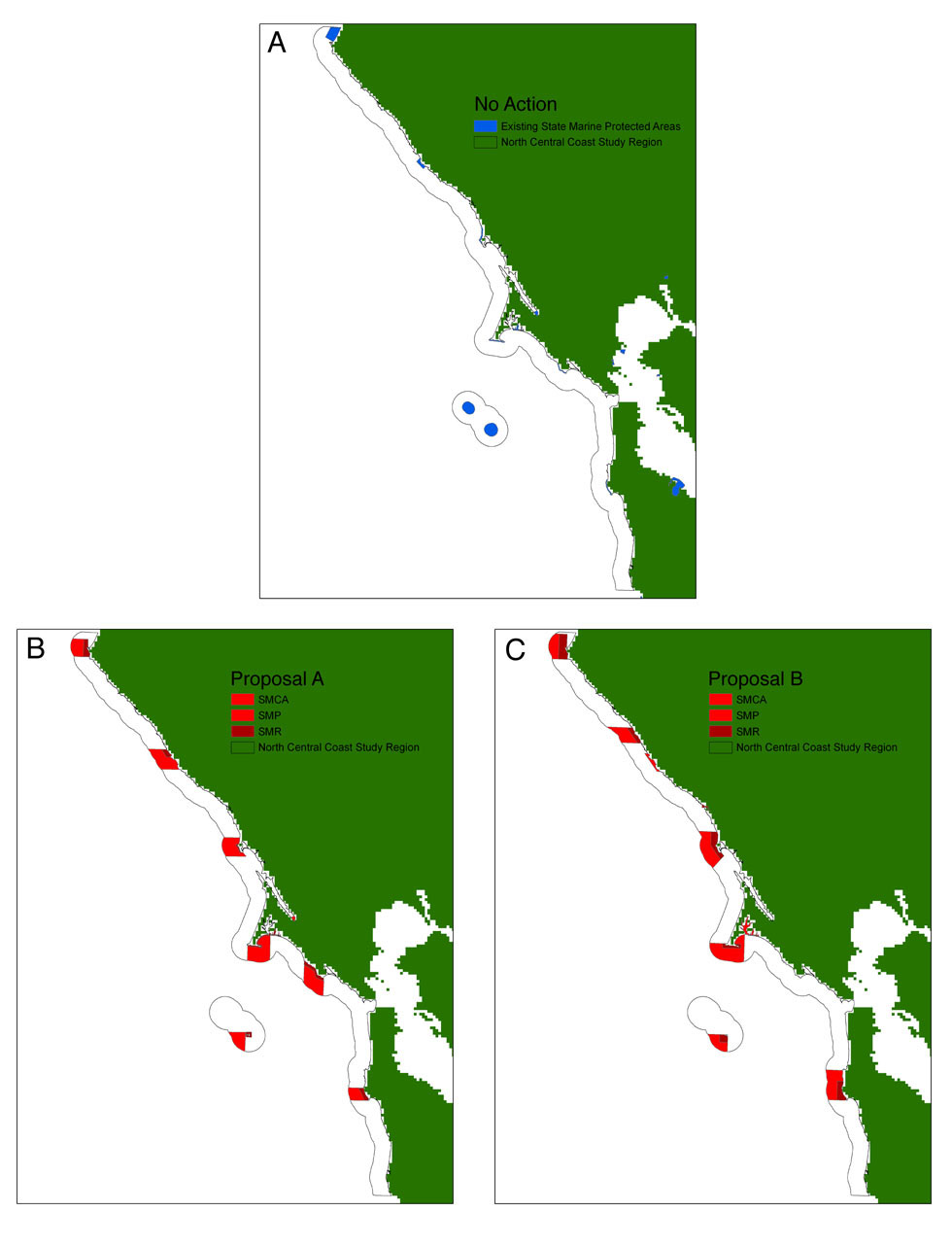
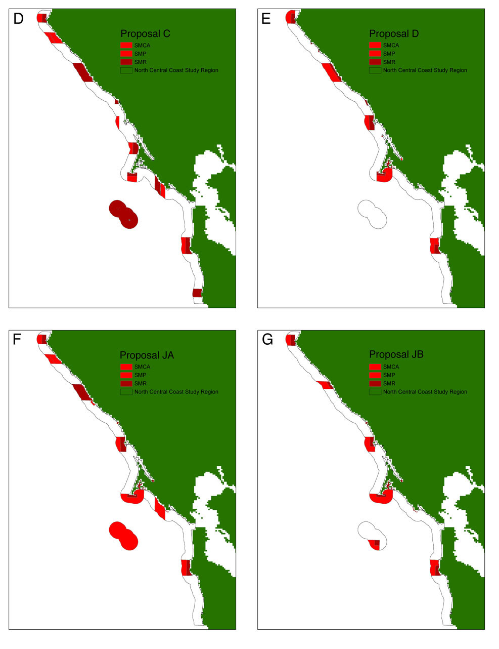
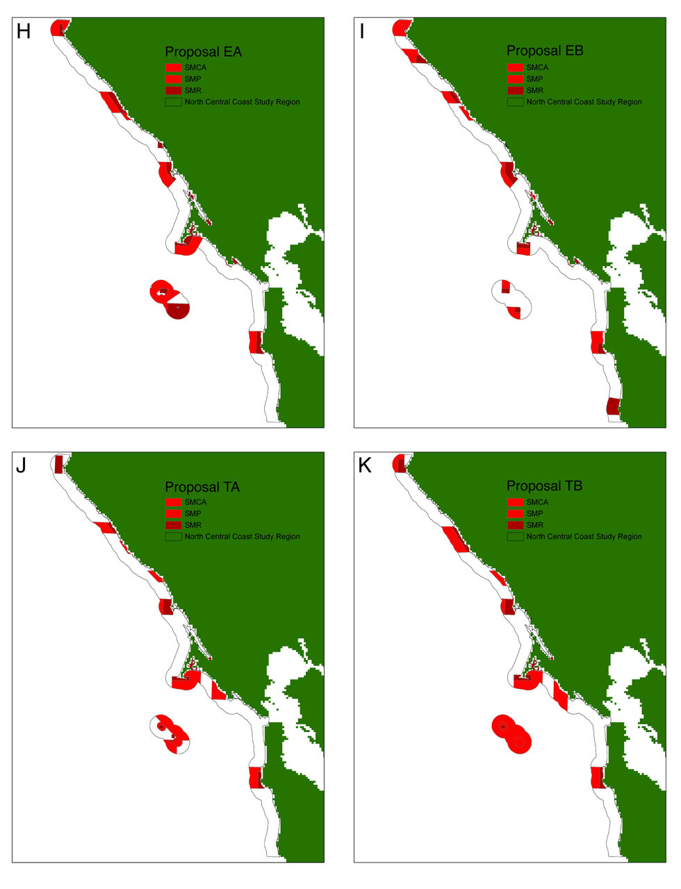
The process for implementing new MPAs under the California Marine Life Protection Act proceeds on a regional basis. Within each study region, local stakeholders propose networks of MPAs; each proposal is evaluated by a committee of scientists, and proposals undergo several rounds of revision by stakeholders and scientific review before being submitted to policymakers for a final consideration. The North Central Coast Study Region (NCCSR) extends from just north of Pt. Arena in the north to Pigeon Pt, north of Santa Cruz, in the south (Fig. C1). For heuristic purposes, we present results for the ten draft MPA proposals submitted at the beginning of the selection process in the NCCSR in October 2007 (Fig. C2). These proposals had not yet undergone scientific review and spanned a wide range of coverage.
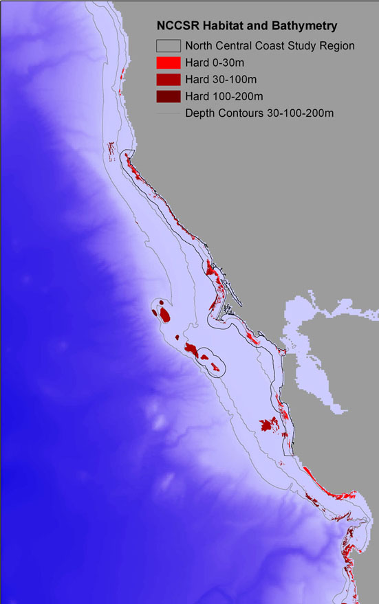
Habitat maps were compiled from three sets of maps available from the California Department of Fish and Game (CDFG): fine-scale substrate maps for state waters in the Central Coast and North Central Coast Study Regions (CCSR, NCCSR) and a statewide, course-scale hard- and soft-bottom habitat map which extends offshore and to the north of the NCCSR. Combining these data sources produced a 407 km × 275 km rectangle that encompassed the NCCSR plus 100 km to the north and south. The upper left (NW) and lower right (SE) corners of the bounding box (California Teale Albers projection, NAD83, meters) were -430000E, 217000N and -155000E, -190000N, respectively. Lat-lon coordinates were: 39° 51'58"N, 125° 1'52"W and 36° 17'40"N, 121° 43'41"W. The maps classified substrate as "hard" or "soft" bottom and classified bathymetry into three depth bins: 0–30 m, 30–100 m, and 100–200 m.
To obtain one-dimensional representations of coastal habitat, we first converted the two-dimensional habitat maps into 1 km × 1 km rasters. We classified cells as "hard bottom" if they were ≥ 50% water and > 40% of mapped substrate in the cell was hard. Depth was assigned as the depth class of the most abundant hard habitat in that cell.
|
|
| FIG. C1. Map of the North Central Coast study region in California (outlined in black) and surrounding areas, showing hard bottom habitat (classified by depth), bathymetry, and boundaries of NCCSR. |
Similar raster files were also generated for each MPA package; in these, a cell was considered to be protected by an MPA if > 25 % of the cell was within the MPA. In general, conversion from two dimensional (2-D) maps to a one dimensional (1-D) model domain proceeded according to a few simple rules, and was done separately for each species in order to account for differences in habitat requirements and MPA regulations. Two types of 1-D domain were created: one describing the presence or absence of habitat, and one describing the protection afforded by an MPA package.
The process was as follows: the 2-D map was divided into latitudinal strips. If at least one cell of suitable habitat occurred within that strip, the corresponding 1-D cell was counted as habitat (1); if not, it was non-habitat (0). Thus the 1-D habitat representation was purely binary (1 or 0).
If at least one cell in the strip contained suitable habitat and was also protected in an MPA, the corresponding 1-D cell was considered to be protected in an MPA. If multiple cells within the 2-D strip met the joint habitat and MPA criteria, the corresponding 1-D cell was assigned the highest level of protection from among those cells within the strip (for example, if a strip contained both an MPA which allowed some harvest and a no-take MPA, the 1-D cell was no-take). For the 1-D representation of MPAs, cells were categorized along a continuum from 0 (no restrictions on fishing) to 1 (no fishing allowed). Some MPAs permitted commercial but not recreational fishing or vice-versa; in those cases we estimated the fraction of the fishery that is of each type and categorized the MPA accordingly. So if the fishery were 50% commercial, 50% recreational, and an MPA allowed recreational fishing only, that cell was coded as 0.5 in the 1-D representation.
These general procedures for converting 2-D strips into 1-D cells were modified somewhat in regions where the coastline deviated from approximate linearity. The coastline north of Pt Reyes and south of Estero de Limantour were treated in the standard way as a linear coastline. The habitat offshore of the tip of Pt. Reyes was approximated as a single 1-D cell by applying the classification rules for latitudinal strips to the group of 2-D cells south and west of the point. The coastline along Drakes Bay was classified using vertical (longitudinal) strips rather than horizontal (latitudinal) strips. The California territorial waters surrounding the offshore Farallon Islands were also modeled as latitudinal strips in the standard way.
Larval dispersal along the linearized coastline was modeled as a function of distance from the point of release, following a Gaussian distribution. For the Farallon Islands, we assumed that larval dispersal from the coastline north of Pt Reyes to the islands was a function of geographical distance in the usual manner. Likewise, dispersal within the island region was a function of distance, but larvae spawned at the islands did not disperse to the mainland and larvae spawned on the mainland south of Pt Reyes did not disperse to the islands.
Because the coastline does not run perfectly north-south, each 1 km-wide 1-D cell actually represented > 1 km of linear coastline. To correct for this, we assumed that each 1 km latitudinal strip represented approximately 1.2 km of linear alongshore distance (this correction factor is calculated as 1/cos(34°), where 34° is the approximate deviation of the majority of the coastline from due north). This corrected alongshore distance was used in all larval dispersal and home range calculations.