Jon S. Horne, Edward O. Garton, Stephen M. Krone, and Jessie S. Lewis. 2007. Analyzing animal movements using Brownian bridges. Ecology 88:2354–2363.

Appendix A. Derivation of Brownian bridge probability distribution when location errors are normally distributed.

Begin with density functions f_a and f_b of the initial and final positions of the Brownian bridge, as well as the variance of the underlying Brownian motion and let

(A.1)

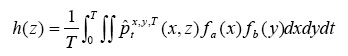
be the expected occupation time density of the Brownian bridge over the time interval [0,T]. Equation A.1 is simplified by considering the spatial integrals. For simplicity, we write out the details in the one-dimensional case; the two-dimensional case is almost identical, but the notation is more cumbersome.

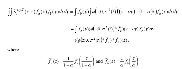
We begin with a few simple observations that will simplify the calculations. Firstly, if f(x) is a density function and K>0 is a constant, then g(x) = Kf(Kx) is also a density function. Secondly, if f(x) and g(x) are density functions, then a simple change of variables shows that

where is the convolution of the densities f and . Such a convolution represents the density of the sum of two independent random variables having the marginal densities f and . Finally, for notational convenience let  = t/T and write

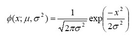
for the density of a random variable.

The three-fold convolution is the density function for a sum X + Y + Z of independent random variables X, Y, Z having marginal densities , , and , respectively. The special case of normal distributions and for initial and final positions simplifies this expression considerably. In this case, it is easy to check that and . Thus,

Plugging this into Eq. A.1, we see that the density of the fraction of time spent by the Brownian Bridge “near z” is

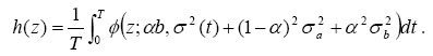
This expression agrees with a conjecture in Bullard (1999).

LITERATURE CITED

Bullard, F. 1999. Estimating the home range of an animal: A Brownian bridge approach. M.S. Thesis. University of North Carolina, Chapel Hill, North Carolina, USA.