Ecological Archives E094-083-D1

Susana Rodriguez-Buritica, Helen Raichle, Robert H. Webb, Raymond M. Turner, and D. Lawrence Venable. 2013. One hundred and six years of population and community dynamics of Sonoran Desert Laboratory perennials. Ecology 94:976. http://dx.doi.org/10.1890/12-1164.1

Introduction

Long-term monitoring of perennial plant populations provides insights into the mechanisms governing community assembly and dynamics. Here, we present data from the longest running individual plant-based permanent plot monitoring project in the world. In 1906, Volney Spalding established 18 permanent plots approximately 100 m² in size on Tumamoc Hill, in Tucson, Arizona, USA. Spalding initially recorded the locations of plant trunks, but in 1910, Forest Shreve began mapping canopy outlines to add to the plant-trunk locations. In 1928, Shreve added 8 contiguous plots totaling 800 m². Although some plots were destroyed by subsequent development, the remaining Spalding-Shreve plots have been periodically monitored since their establishment, resulting in a set of detailed maps depicting species location and canopy coverage, as well as a set of repeat photographs capturing plant community changes that have occurred over the last century.

Analyses of the Spalding-Shreve plots have greatly contributed to our understanding of plant community dynamics in general and Sonoran Desert plant communities in particular. At the beginning of last century, when Clements’ ideas of a superorganism started to take shape (Clements 1916), the analysis of between 8 to 30 years of change in Spalding-Shreve plots represented an excellent opportunity to test Clements’ paradigm (Shreve and Hinckley 1937). The lack of directional changes in community attributes was an indication that vegetation changes were controlled by a number of interacting conditions (Shreve and Hinckley 1937) and were not progressing towards a climax community, as would occur under Clementsian succession. Subsequent analyses by Murray (1959) and Bowers (2002 and 2005 a,b) demonstrated that these interacting conditions include species-specific climate control on recruitment and mortality and herbivory pressures that could decouple demographic and climatic trends. Goldberg and Turner (1986) found that although there were no consistent directional changes in vegetation composition after 72 years, sharp difference in species-specific dynamics were apparent, suggesting that long-term community dynamics is highly sensitive to exceptional climatic events (either wet or dry). In addition, by investigating the fate of individual plants over 72 years, Goldberg and Turner (1986) were able to estimate survival and lifespan for common species and to demonstrate clear correlations among several life-history traits. Most recent analyses of this dataset indicate that positive plant-plant interactions can buffer effects of low- and high-frequency climatic variations, leading to a decoupling between climatic and plant-community trajectories (Butterfield et al 2010). Munson et al. (2012) combined the Spalding-Shreve data set with others in the region to relate changes in plant abundance to climate variability and predict future shifts in plant community composition. In this data paper, we present the full set of maps derived from censuses on Spalding-Shreve plots between 1906 and 2012. The archiving process was conducted in two stages. In 2001, the paper-map data were digitized; starting in 2010, data were compiled and subjected to strict quality control. Scans of original maps are provided along with digitized versions of plant-trunk locations, and plant-canopy outlines. In addition, we are providing a comprehensive enumeration of all available material related to these plots and their current location, including a digital version of Spalding’s unpublished notes (see section Table 7 for information on status and location of these notes); secondary, nonspatial information of the plots (plant heights, list of annuals, notes on disturbance); and a list of all photographs that show these plots.

Metadata

Class I. Data set descriptors

A. Data set identity: Title: 106 years of population and community dynamics of Sonoran Desert perennial plants at the Desert Laboratory (Tucson, Arizona).

B. Data set identification code: NA

C. Data set description

Originators: I.C.1. Originators: Raymond M. Turner, 5132 East Fort Lowell Road, Tucson, AZ 85712, [email protected] and Robert H. Webb — U.S. Geological Survey, 520 N. Park Avenue, Tucson, AZ, 85719, [email protected].
Archivists include H. Raichle — U.S. Geological Survey, 520 N. Park Avenue, Tucson, AZ, 85719, [email protected] – and Susana Rodriguez-Buritica —Department of Ecology and Evolution Biology, University of Arizona. Tucson, AZ 85701, [email protected].

Abstract: This data set constitutes all information associated with the Spalding-Shreve permanent vegetation plots from 1906 through 2012, which is the longest-running plant monitoring program in the world. The program consists of detailed maps of all Sonoran Desert perennial plants in 30 permanent plots located on Tumamoc Hill, near Tucson, Arizona, USA. Most of these plots are 10 m × 10 m quadrats that were established by Volney Spalding and Forrest Shreve between 1906 and 1928. Analyses derived from this data have been pivotal in testing early theories on plant community succession, plant life history traits, plant longevity, and population dynamics. One of the major contributions of this data set is the species-specific demographic traits that derived from estimating individual plant trajectories for more than 106 years. Further use of this data might shed light on spatially explicit population and community dynamics, as well as long-term changes attributable to global change. Data presented here consists of digital versions of original maps created between 1906 and 1984 and digital data from recent censuses between 1993 and 2012. Attributes associated with these maps include location and coverage of all shrubs, and, in some cases, plant height. In addition, we present plot-specific summaries of plant cover and density for each census year and all other information collected, including seedling counts, grass coverage, and annual species enumerations. We reference the repeat photography of these plots, which began with original photography in 1906; these images are stored at the Desert Laboratory Collection of Repeat Photography in Tucson. Initial data collection consisted of grid-mapping the plots manually on graph paper; starting in 1993, Total Stations (which allow a direct digitalization, and more accurate mapping) were used to survey root crowns and canopies.

D. Key words: Arizona; community dynamics; longevity; long-term monitoring; permanent plots; population dynamics; Sonoran Desert; vegetation change.

Class II. Research origin descriptors

A. Overall project description

Identity: Long-term monitoring of Sonoran Desert perennial plant communities at the Spalding-Shreve Plots at the Desert Laboratory (Tucson, Arizona).

Originator: V. Spalding and F. Shreve, Desert Botanical Laboratory (between 1906 and 1928). More recently project has been lead by Raymond M. Turner -5132 East Fort Lowell Road, Tucson, AZ 85712, [email protected] and R. H. Webb —U.S. Geological Survey, 520 N. Park Avenue, Tucson, AZ, 85719, [email protected].

Period of Study: 1906–2012

Objective: To monitor cover and density of perennial plant communities in the Sonora Desert.

Abstract: see above.

Sources of funding: Carnegie Institute of Washington; U.S. Forest Service, U.S. Geological Survey; University of Arizona; National Science Foundation DEB 0817121 (LTREB) to D. L. Venable.

B. Specific subproject description

1. Site description:

Site type: Tumamoc Hill rises 245 m above the surrounding alluvial plain to an elevation of 960 m (a.s.l.); it is within the 3.52 km² of the Desert Laboratory owned by the University of Arizona. Vegetation of the Desert Laboratory is characteristic of the Arizona Upland Division of the Sonoran Desert (Goldberg and Turner 1986).

Geography: The Desert Laboratory is located about 2 km west of downtown Tucson, Arizona (32° 13' 12.281' N, 111° 0' 16.098' W) on an outlier volcanic outcrop of the Tucson Mountains. Slopes at the Desert Laboratory ranges from predominantly gentle on the lower north aspect (mean = 63%) to steep along the south (mean = 109%) and east (mean = 129%) aspects.

Habitat: Vegetation on Tumamoc hill is characteristic of Arizona Upland Division of Sonora Desert (Goldberg and Turner 1986). Dominant vegetation includes Cercidium microphyllum (Torr) Rose & I.M. Johnson, Carnegiea gigantea (Engelm.) Britt & Rose, Larrea tridentata (Moc & Sess) Cav. Fouquieria splendens Engelm., Ambrosia deltoidea (A. Gray) Payne, Encelia farinosa A. Gray, Aloysia wrightii (A. Gray) Heller, Opuntia engelmannii Salm-Dyck, and Ferocactus wislizeni (Engelm.) Britt & Rose as dominant species. The file Plots.csv provides plot-specific descriptions as observed by Spalding in 1906.

Geology: Tumamoc Hill is dominated by volcanic rocks (Spencer et al. 2003), mostly Tumamoc basaltic andesite (middle Tertiary: ~23–24 Ma) along the north slopes and at the higher elevations along all other three sides of the mountain. At upper and middle slopes on the west, south, and east sides, the rocks are Tumamoc tuff (middle tertiary: ~ 26–28 Ma) and a conglomerate (~26–28 Ma). The lower slopes are dominated by Mafic volcanic rocks (early Tertiary or late Cretaceous), particularly on the west side, and basaltic andesite (~26–28 Ma). A large area of the Desert Laboratory to the west consists of colluvium and alluvium of mostly Quaternary Age dissected by washes (Webb and Turner, 2010). Soils on steep slopes generally are shallow and are clay soils with petrocalcic horizons and surficial colluvial basalt boulders. Sandy soils relatively free of rocks dominate the lower slopes (Phillips 1976). Many of the soils on higher geomorphic surfaces are middle Pleistocene to late Tertiary in age and have surfaces littered with caliche rubble that originated in petrocalcic horizons.

Watershed/hydrology: Tumamoc Hill is drained by small ephemeral washes that form high-angle chutes on the steepest slopes of all four sides. Silvercroft Wash, with its headwaters west of the Desert Laboratory, passes across the northwestern quarter of the grounds. The alluvial landscape that constitutes the western half of the property is mostly attributed to sedimentation by this ephemeral wash. None of the Spalding-Shreve plots is situated in a xeroriparian setting.

Site history: The Carnegie Institution of Washington established the Desert Botanical Laboratory (352 ha) in 1903. In 1907, the property was fenced in to exclude livestock grazing and prevent the extraction of rocks and vegetation (Shreve 1929), which had been occurring since 1858. This fencing means that the Desert Botanical Laboratory grounds represent the longest known restoration ecology site in the world (M. Rosenzweig, personal communication, 2011). In 1940, the Carnegie Institution transferred the property to the U.S. Forest Service, which sold it to the University of Arizona in 1956. At some unknown point in time, the name was shortened to Desert Laboratory. Further information about the history and other long-term projects at the Desert Laboratory can be found in Bowers (2010) and Webb and Turner (2010).
Disturbance History: Several disturbances have affected plant community dynamics on the Desert Laboratory, including direct disturbances of some of the Spalding-Shreve plots that led to partial or complete plot destruction (see file Plots.csv for details). All plots had some amount of livestock grazing disturbance prior to fencing of the property in 1907. Road construction at various times is the main culprit in disturbing or destroying plots. In 1933, 1955, 1981, 2003, and 2004, several areas of the property were disturbed by the installation and subsequent replacement of gasoline and natural gas pipelines (Fig. 1). Here, we summarize the major events based on a compilation by Janice Bowers in 2002, which can be found in the files at the Desert Laboratory on Tumamoc Hill. Specific information regarding disturbance at each of the permanent plots is summarized in the file Plots.csv.

1. Evidence of human activities at Tumamoc Hill date back to ca. 2300 years ago and suggests an early agricultural period (Wallace et al 2007); at this time indigenous peoples build a town at the top of the hill that was surrounded by a trinchera (massive dry-laid masonry walls). During pre-columbian times, the Hohokam occupied Tumamoc hill leaving evidence of an extensive use for residence, farming, and ceremonial activities (A.D. 850–1300 –Wallace et al 2007). Between ca. 1450 and 1757 occupation and use of Tumamoc hill diminished; at the end of this period new colonial settlements are established near Tumamoc Hill and the city of Tucson is founded (1775).
2. Light cattle, horse, goat, and burro grazing between 1858 and 1907. Stocking rates are unknown.
3. In 1907, property was fenced and protected from grazing as well as removal of rocks and native plants.
4. In 1933, El Paso Natural Gas installed a natural-gas pipeline with a 9.14 m wide easement across the northeast side of the property.
5. In 1955, Southern Pacific constructed a 15.24 cm wide natural gas pipeline and a 20.32 cm wide petroleum pipeline (See Fig. 1 for details) along with a 12.19 m wide easement on the west side of Tumamoc Hill. Kinder Morgan Energy Partners (KMEP) now owns this pipeline.
6. In 1981, a flood-control dike was constructed east of Silvercroft Wash and south of Anklam Road (Fig. 1).
7. In 2003, KMEP installed a new 30.48 cm wide pipeline. The total construction easement was 27.43 m wide, although a narrow strip along the eastern edge of the easement was not re-disturbed. Cacti and ocotillos (O. engelmannii, Cylindropuntia versicolor (Engelm. Ex Toumey) F.M. Knuth, C. fulgida (Engelm), C. kleiniae (DC.) F.M. Knuth Carnegiea gigantea, F. wislizeni, Echinocereus fasciculatus (Engelm. Ex B.D. Jacks.) L.D. Benson, Mammillaria grahamii Engelm., F. splendens.) were salvaged from the easement and re-planted in 2004 along the easement. Except for the northernmost section (approximately 200 m in length), the entire easement was hydroseeded with seeds of shrubs and short-lived perennials.
8. In August 2003, El Paso Natural gas replaced portions of the pipeline and installed a launcher station at City Gate #1. A section of easement about 192 m in length and 9.6 m in width was cleared of vegetation. F. splendens, cacti (O. engelmannii, C. versicolor, E. fasciculatus, F. wislizeni, C. gigantea, M. grahamii), and shrubs and trees (Prosopis velutina Wooton, Cercidium microphyllum, Acacia constricta A. Gray, F. splendens) were salvaged and replanted.
9. In January 2004, the El Paso Natural Gas revegetated the easement. Salvaged plants were transplanted along with shrubs and cacti (A. deltoidea, L. tridentata, Krameria grayi Rose & Painter, F. splendens, O. engelmannii, C. versicolor) from a nursery. Salvaged shrubs and trees were transplanted to the outside edge of the easement. In mid-January 2004, the easement was hydroseeded with seeds of shrubs and short-lived perennials. The seed mix included warm-season and cool-season germinators.
10. Between 2004 and 2005, El Paso Natural Gas easement was sprinkler-irrigated. A series of matched photographs (Stake 905 in file Stake_Info.csv) taken in 1958, 1978, and 2003 show that considerable recovery occurred on the easement between 1955 and 2003.
11. In 2005, drilling was conducted along the flood-control dike, causing local, light damage; shrubs and cacti were crushed by heavy equipment, and the ground was rutted where vehicles drove.

Climate: Mean annual precipitation at Tumamoc Hill is approximately 298 mm, with 36% of precipitation occurring between November and March and 53% occurring between June and September (Webb and Turner, 2010). Considering the decadal variability in precipitation, Turner (2003) identified two wet and two dry periods affecting the Desert Laboratory since 1906 (shades in Table 1). The two wet periods are from 1906 to 1940 and from mid 1970s to 1998, while the drought periods were from the mid-1940s to early 1960s and the 12 years following 1999 (Turner et al. 2003).

2. Experimental design:

Area selection

In 1906, V. M. Spalding established eighteen 10 × 10 m and two 1 × 1 m permanent plots in several habitats on the Desert Laboratory grounds. The reason for the exact plot locations is unknown, but they appear to represent the dominant plant communities at the Desert Laboratory (Spalding, unpublished notes, 1906). The purpose of these plots was to record changes in perennial and annual plants through time. The two 1 m × 1 m plots were designed to monitor yearly changes in annual plants (Shreve 1929), but data collected from these plots could not be located for archiving. When the 10 m × 10 m plots were established, one of the main objectives was to monitor the recovery of plant populations after grazing was excluded from the Desert Laboratory grounds in 1907 (Shreve 1937). Some plots were established for the purpose of following specific species through time or to illustrate particular growing conditions of plant communities (See file Plots.csv for details). Once the site of each plot was selected, Spalding permanently marked the corners with four stakes around which stones where piled. Later, these markers were replaced by metal rods set in concrete (Shreve 1937). Later still, missing corner markers were replaced with rebar or aluminum angle iron. As a result, several different corner markers are now present on some plots. Nevertheless, the loss of some markers has prevented the re-location of some plots (plot 8 and 17), as well as the spatial precision of some censuses in the remaining plots (see Plots.csv)

Between 1910 and 1928, F. Shreve established two additional areas of observation; one with the purpose of monitoring annual seedling establishment and changes in several shrub species (area A, established in 1910, Fig. 1), and the other with the purpose of monitoring grass establishment (area B, established 1928; Shreve 1937, Fig. 1). The latter area consists of eight contiguous 10 m × 10 m plots for a total of 800 m², which was extended in 2010 to 0.1 ha by adding two additional 10 m × 10 m plots, See file Plots.csv for a detailed description of the plots and Section IV.B for an explanation of the file variables.

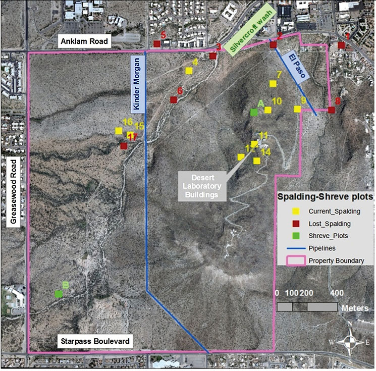
Fig. 1. Known and approximate locations of Spalding-Shreve permanent plots at Tumamoc Hill. Of the original 19 Spalding plots, only 16 have current or approximate locations. Some locations of lost plots (red symbols) were approximated using repeat photography. Location of plots 18–19 could not be determined, although plot 19 corresponds to a denuded 1 × 1 m plot; there is no information regarding plot 13. The map also shows the current boundary of the Desert Laboratory (property boundary) and the location of pipelines along which major disturbance took place.

Data collection period and frequency

Remeasurement of Spalding-Shreve plots involved two activities: (1) censusing plants by a survey method and (2) photographing the plots. During a census, one or several of the following were recorded: presence/absence of all perennial species as previously discussed, location of root bases for each individual plant, and measurement of canopy for each individual plant. Repeat photography used standard methods to locate the original camera station(s) for plot photographs, mark those locations (generally with rebar), and replicate the image. The following sections describe the methods used during plant censusing and repeat photography. Goldberg and Turner (1986) and Webb and Turner (2010) offer a more detailed account of data-collection history.

Plant density and cover

Censuses have been mostly conducted in the winter months of November to April (Shreve 1937). Table 1 summarizes data collection schedules, and Table 2 specifies the dates of each census. Spalding and Shreve avoided annually mapping on these plots because, at the time (between 1906 and 1937), they were monitoring plant community recovery after grazing prohibition, and they preferred to wait until the vegetation more completely recovered from the disturbance (Shreve 1937). Since then, mapping of annuals ceased (except for a presence/absence enumeration in 1983) and perennial censuses have been conducted at irregular intervals. For details about the kind of data collected at each census see Section II.B.3.

Plot photographs

In addition to mapping perennial shrubs, Spalding and Shreve photographed several of the plots using large-format cameras with plate-glass or flexible-film negatives. In many images, the plot number and date were printed directly onto the negative. These images, both negatives and prints, were part of the larger collection of imagery stored at the Desert Laboratory. In the 1950s, Raymond M. Turner made prints from the original negatives or, in some cases, copy negatives from prints for which the negatives had been lost, and began replicating the images. Matching of old photographs began in 1960, when James R. Hastings and R. M. Turner used repeat photography to study bioclimatology of vegetation change in the Sonoran Desert (Webb et al. 2007), including the Desert Laboratory. In addition to matching the photographs from Spalding-Shreve plots, Turner established new photographic stations for plots for which there were no original images. Since then, repeat photographs have been taken in parallel with census efforts. For more details about repeat photography procedures see Section II.B.3.

Table 3 summarizes the number and frequency of photographs taken on the Spalding-Shreve permanent plots. Files Stake_Info.csv and Photo_Info.csv summarize details associated with each matched photograph. Photographs are permanently stored as part of the Desert Laboratory Collection of Repeat Photography. Figure 2 provides a sample of the post-processed matches for plot B7.

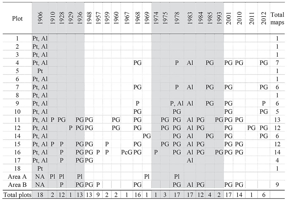
Table 1. Census schedule for Spalding-Shreve plots. For each cell, the presence of letters indicates that a census was conducted (see Section II.B.3 for a detailed description on data collection). Capital letters indicate which functional group was censused: P = perennial plants except grasses, A = annuals, G = perennial grasses. Lowercase letters indicate the data type recorded: l = list of species but not canopy outlines, t = only root crowns (part of the root system from which stem rises) were mapped, c = all canopies but not all root crowns were mapped, P (without t or c data type descriptor) = both canopies and trunks were mapped. Plot 13 and 19 were excluded from this table; there is no information regarding plot 13, which presumably correspond to one of the 1 m × 1 m plots. Plot 19 was the other 1 m × 1 m plot; it was denuded area, and there was no information about this plot except a photograph taken in 1906. Shading indicates years considered within the wet decadal periods (Turner 2003, Webb and Turner 2010)

Table 2. Specific dates for each census of the Spalding-Shreve plots. Rows indicate the years plots were read and columns designate plots. Dates within cells indicate the month and the day when censuses were conducted (mm.dd). Dates within parenthesis correspond to additional census dates when census on annuals or grasses (dates with a preceding “g”) were conducted; X is used when specific dates are unknown. A single number indicates the month of the census in cases when no information about the specific days was available. Shading indicates years considered within the wet decadal periods (Turner 2003, Webb and Turner 2010).

Table 2 continued. Specific dates for each census of the Spalding-Shreve plots. Rows indicate the years plots were read and columns designate plots. Dates within cells indicate the month and the day when censuses were conducted. Dates within parenthesis correspond to additional census dates when census on annuals or grasses (dates with a preceding “g”) were conducted; X is used when specific dates are unknown. A single number indicates the month of the census in cases when no information about the specific days was available.

Year	17	18	B1	B2	B3	B4	B5	B6	B7	B8	B9	B10
1906	03.1 (4.2)	3.7 (3.7)
1928	12.2		X	X	X	X	X	X	X	X
1929
1936	2.24		3.16	3.17	3.16	3.1	3.4	3.17	3.4	3.1
1948	X		X	2.13	X	3.4	2.14	X	X	2.28
1957			3.26	4.8	4.22	4.12	4.25	5.16	4.27	6.3
1968			1.12	1.12	1.12	1.12	1.15	1.15	1.15	1.15
1978			2.15	3.27	2.22 (g3.22)	3.23	3.28	3.29	3.28	3.29
1983	4.22		4.18	4.18	4.18	4.18	4.18	4.18	4.18	4.18
1984			6.1	6.1	6.14	6.14	6.14	6.15	6.14	6.15
2001			5	5	5	5	5	5	5	5
2010			4.28	4.28	5.4	5.5	4.29	4.29	5.4	4.29	5.5	5.5

3. Research methods:

Field protocol

Different methods have been used to census plants growing inside each of the Spalding-Shreve plots. Between 1906 and 1978, the census protocol broadly consisted in mapping the location of each perennial shrub. As a guide in this process, censuses were conducted using a cord grid to divide the plot into one-meter squares. Cords were placed near the ground when possible or in rare occasions, over a plant’s canopy with the help of pins to secure the location of the rope before and after the canopy (Goldberg and Turner 1986). Mapping was done on graph paper on which the meter squares were divided into square decimeters (dm²). In 1906, plant trunks were mapped on graph paper at a scale of 1 cm = 1 m on the ground (1:100 scale; Spalding, unpublished notes, 1906). Later, this procedure was done using 25.5 cm x 25.5 cm graph paper so the scale used was 2.55 cm = 1 m on the ground. In 1984–1985, a plane table and alidade were used for mapping and final maps were generated in Mylar-type film. There is no specific information on the procedures used in these censuses. Previous to 1985, plots were represented as squares of 10 m on each side; nevertheless, when a Total Station was used in later censuses, it was evident that some of the plots were not squares. For details on corrections associated with this issue see Section  V.E.

Starting in 1993, a total station (TS), which incorporates a laser electronic distance meter (EDM), was used in combination with a reflector prism mounted on a stadia rod to record the position of the trunks and the size of the canopies. Theoretically, the accuracy of each surveyed point is on the order of millimeters, but practically, survey data is probably accurate to the footprint of the stadia rod (around 2–4 cm). For each plant, the base of the root crown and a few points along the canopy border were recorded.

Independent of the instruments used, in every census, the plants rooted inside the plots were mapped with the location of root crown and canopy outline. For plants rooted outside the plots, only the part of the canopy inside each plot was mapped. In general, only living plants were mapped. If dead plants were mapped, they were labeled as such. In the following section we summarize the particular criteria using during each census.

Specific criteria used during each census

In the following paragraphs, we describe the variations over the general protocol and any specific criteria used during particular field censuses. Information for this section was extracted from unpublished field notes and personal notes, draft and final maps, and publications.

In 1906, all perennial plants were mapped except Dichelostemma capitatum Alph. Wood due to the difficulty seeing all individuals of this geophyte in the quadrat (Spalding, unpublished notes, 1906). Spalding mapped the annual alfilerilla or filaree (Erodium cicutarium –L.- L’Hér. Ex Aiton) to monitor its invasion; while Chamaesyce capitellata (Engelm.) Millsp. was not mapped because it was not recognized as a perennial at the time. In addition to mapping the position of the trunks, all perennial species were identified and their heights categorized in accordance with Table 4. Finally, Spalding listed the annual species present at the time of the census with some notes on their abundance. This information is summarized in file Count1906.csv

Table 3. Number of photographs taken of Spalding-Shreve plots. Numbers in each cell are the total number of photographs associated with each plot, which includes photographs from different stations and different photographs at the same station.

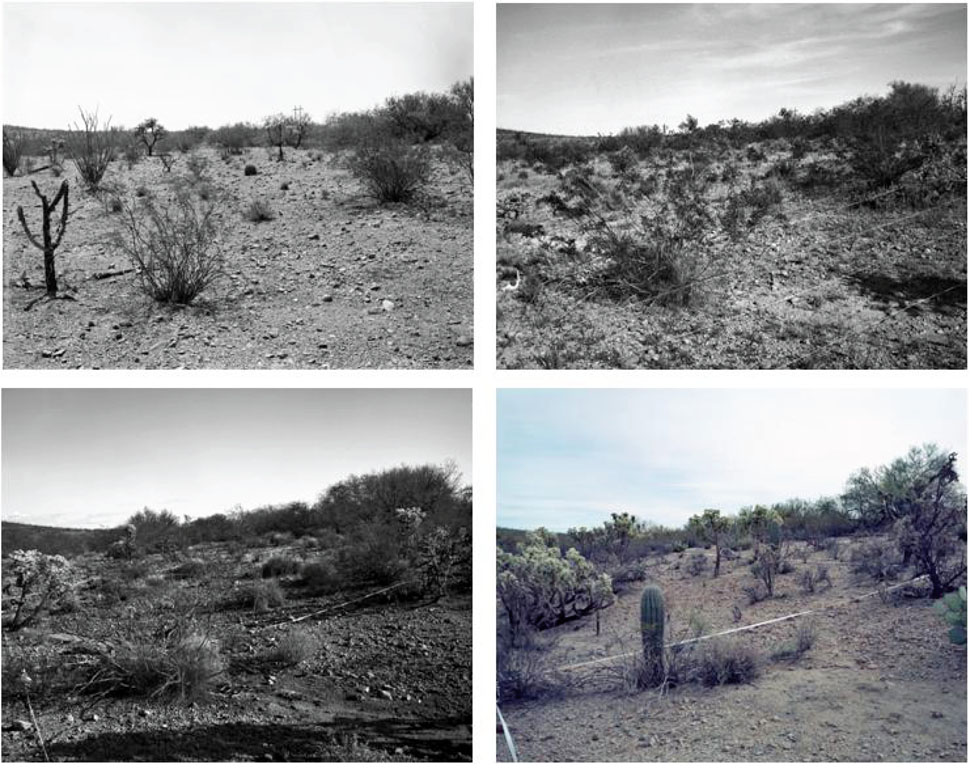
Fig. 2. Sample of matched photographs for plot B7. Photographs were taken from stake 912 and processed according to matching protocols explained in section II.B.3. Photos were taken in 1958 (upper-left panel), 1978 (upper-right), 1986 (lower-left), and 2009 (lower-right). For information about available photographs see section IV.A.1

Table 4. Height categories used by V. Spalding during the 1906 census. Information derived from Spalding (unpublished notes, 1906).

Between 1910–1936, censuses did not include bulbous or herbaceous perennials that are hard to identify in the dry months, such as Delphinium scaposum Greene and Anemone decapetala (Poepp.) Ard. This criterion was also applied in censuses between 1968 and 1985, as well as during censuses between 2010 and 2012. Although there is no explicit documentation, this criterion was probably applied in all other censuses between 1948 and 1968 as well as in 2001. Despite the criterion, when censuses were conducted later in the spring, some species regularly excluded were mapped wherever present (e.g., 1978). Care should be taken in statistics derived for species with a highly sensitive detection threshold (e.g., Sphaeralcea grossulariifolia (Hook. & Arn.) Rydb., Glandularia gooddingii (Briq.) Solbrig.,and Ayenia pusilla L.). Carlowrightia arizonica A. Gray, Haplophyton cimicidum A.DC., Menodora scabra Engelm. Ex A.G., and Siphonoglossa longiflora (Torr.) A. Gray are difficult to distinguish and they never appear together in some plots, which suggests potential misidentifications (Goldberg and Turner 1986). See file Species.csv for description on the quality of plant identifications throughout the censuses.

Other information has been recorded in some censuses but not in others (Table 5), including: information on the size of root crowns, explicit recognition of plant clusters for which individual canopies cannot be determined (e.g., Calliandra eriophylla Benth. or Tiquilia canescens (A. DC.) A.), explicit identification of seedlings, recording of dead plants or dead parts of plants, and grasses (e.g., Aristida sp., Bouteloua sp., Pleuraphis sp.).

In area B, Aristida glauca (Nees) Walp, Aristida ternipes Cav., along with Digitaria californica (Benth.) Henrard, Sporobolus R. Br., Pleuraphis sp. Kunth, and Muhlenbergia porteri Scribn were only explicitly mapped in 1936, 1948, 1968, 1978 (R.M. Turner’s unpublished notes), and in 2010.

The height of some species was recorded on the map in 1906, 1928, 1936, 1960, 1968, 1975, 1978, 1984, and 1985; measurements were typically done for large plants like L. tridentata, F. splendens, A. constricta, P. velutina, C. microphyllum, and C. gigantea. This information is included in the files *trunks.shp.

In the 1948 census, field notes included measurements of height and notes on general condition of all plants; from these notes, dead and new plants can be clearly identified, as well as plants with multiple trunks. This information is included in the file *trunks.shp and *crowns.shp

In 1957, all perennials were mapped except perennial grasses and Baileya multiradiata Harv. & Gray, Ditaxis lanceolata (Benth.) Pax and Hoffman, and Bahia absinthifolia Benth. Seedlings of Psilostrophe cooperi (A. Gray) Greene were not mapped. In addition, large canopies at the border of two contiguous plots were only mapped for the plot where the root crown was located (Murray, unpublished notes, 1957 –see Table 7 for location of these notes). During the archiving process, we completed the polygons representing the canopy of these plants so each plot map has all the plants with canopies inside each plot (see Section V.E for details).

There is no specific information about mapping protocols for 1984–2001 censuses, but maps only contained perennial species. Seedlings and clusters were not explicitly identified, and dead plants/parts were not recorded.

In 1993, some plant canopies were approximated using ellipsoids. For this purpose, instead of mapping the canopy perimeter, researchers measured the maximum length (a) and the length perpendicular to the maximum (b) and estimated canopy area using the equation (A=πab/4). During archiving in 2010, these ellipsoids were converted to a circle of diameter given by the squared root of 2A/π because the directions of the a and b diameters was not recorded. These plants are explicitly identified as PointCircles in the attribute table (see Section IV.B.6). See Section V. E.1 for more details on the archiving process. In addition, for all plants with canopies inside the plot, the entire canopy was clipped to plot borders during post-census processing in 2010.

In 2001, mapping was conducted in three steps. First, the size and location of each perennial plant was recorded using a total station (TS) surveying instrument. At least 4 points were taken around the perimeter of each plant’s canopy; but for small plants only 2 points were taken, and in some cases only the root crown. In this last case, plants were referred to as points (see Section V.B) and usually represent seedlings, although they were not explicitly recognized as such. In a second step, canopy points recorded by the TS were connected and smoothed by hand in the field. (see Instrumentation below for more information about census protocols). Finally, these hand-drawn canopies were then digitized in ArcView and clipped to plot borders. Only living plants and latent plants were included. Grasses were not censused.

During 2010–2012 censuses TS was also used during surveys. The survey was conducted with one person operating the instrument, a second person keeping track of the plant being measured by the TS, as well as recording additional information on each plant (height and diameter), and at a third person handling the prism. In these years, the following mapping protocols were used: only perennial shrubs and grasses were included, and only live plants were mapped. For each mapped plant, the root crown and at least 3 points were recorded for the canopy; the final number of points taken was such that the overall canopy shape was fully captured. For plants whose canopy could be approximated by a regular geometric figure (usually a circle), no canopy points were recorded; instead, diameter was measured and later used to approximate the canopy as a circle or, in one case as a rectangle, centered at the root crown location. These plants are explicitly identified as PointCircles (or PointRectangle) in the attribute table (see Section IV.B.6). For saguaros (C. gigantea), only the perimeter of the trunk was mapped—the trunk was always approximated as a centroid (see Section IV.B.6 for details about centroid estimations). For plants rooted outside the plot, the canopy inside the plot was mapped and extended several decimeters beyond the plot border, but later clipped to the plot border. Seedlings were mapped as points, although they were not consistently identified as such. In plots with mass germination/establishment of certain species, notably Encelia farinosa, groups of seedlings were collectively mapped and described; the area of each cluster was approximated by a circle with a field recorded diameter. See Section V.E for details of the processing of this data during the archiving process. In 2010–2012, height of all plants was measured as the length between the root crown and the top of the tallest live, vegetative branch.

Table 5. Year-specific information collected during Spalding-Shreve censuses.

Repeat photography protocols

In 1906, V. Spalding photographed each of the permanent plots that he established, and his notes describe where the photograph was taken. Since the plots were established, several photographs have been taken from near exactly the same location as Spalding’s photographs. Photographs taken before 1960 did not have written descriptions of how the photograph was taken, so the process of matching the photograph relies only on photointerpretation.

Since 1960, Turner has photographed most of the Spalding-Shreve plots from the original locations. Matching the original photographs entailed first locating approximate where the original was taken, and following parallax principles to established the original location of the camera station (Webb et al. 2010). Once the correct location of the camera station was determined, the site was permanently marked using a metal stake, large nail, or cairn. For each station geographic coordinates were determine by either reading a topographic map, or in recent years by using a hand-held global positioning system (GPS) receiver. For each replicate photograph the azimuth (or bearing) of the view, the camera’s vertical tilt and height above ground level were recorded as well as the camera model, lenses, filters, film numbers, exposures, date, time, names of photographer, and crew. Figure 2 documents the available photographs. Files Stake_Info.csv and Photo_Info.csv compile the detailed information about each photograph in the collection. See section III.B.2 for contact information regarding this collection.

Instrumentation

The following section summarized the specifics of the instruments used during each census (Table 6).

Table 6. Attributes of Instruments used to census Spalding-Shreve plots. More detailed information about the camera used for each of the repeat photographs can be found in file Photo_Infor.csv

Taxonomy and systematics:Throughout this document and in all files associated with this project, we have used the accepted nomenclature reported in Taxonomic Name Resolution Service v3.0 (2012; abbreviated as TNRS for the rest of the document). In addition, file Species.csv, which summarizes the taxonomy treatment of species during the census, also includes the corresponding species codes reported in PLANTS database (USDA 2012). For more information on the flora of the Desert Laboratory, see Bowers and Turner (1985).

Permit history: No permits are required for work at the Desert Laboratory. Permission from the Science Coordinator is necessary to ensure that measurements are made in accord with the accepted protocols for measurement and archiving of data.

Legal/organizational requirements: No additional legal or organizational requirements are necessary beyond coordination with the Science Coordinator.

Project personnel:Table 5 summarizes the people involved in each census. This information was compiled by J. Bowers around 2004 and was updated in March 2012.

Class III. Data set status and accessibility

A. Status

Latest update:November 2012

Latest Archive date:November 2012

Metadata status:November 2012

Data verification:November 2012

B. Accessibility

Storage location and medium:

Table 7 summarizes the location and medium of field notes, maps, and summary tables for each census. Specific information about how this data was archived can be found in section V.E

Table 7. Storage location and medium of all material related to the Spalding-Shreve permanent plots. Nomenclature: SCUA = Special Collections at Main Library of the University of Arizona, Tucson Ref: AZ560 Box 30; USGS = R. H. Webb project, USGS, Tucson Arizona; DLC = Tumamoc Hill Library of the University of Arizona, Tucson.

Repeat photography

Copies of the prints (or printouts), field notes, and any other relevant information are stored in the Desert Laboratory Collection of Repeat Photography at the USGS in Tucson, Arizona. Electronic copies of images are stored both as non-manipulated, high-resolution master TIF file (LZW compression) as well as the digitally matched final version, saved as a 300 dpi/10" wide TIF file (LZW compression). Not all of the images have yet been scanned.

The original Spalding and Shreve negatives are at the Arizona Historical Society (Southern Arizona Division, Tucson) and University of Arizona Special Collections Library (Tucson). All of the matches, and any of the new views established by Turner, are part of the Desert Laboratory Collection of Repeat Photography. All of the images are within the public domain and have unrestricted use beyond proper attribution of photographer and source. Credit information should include stake number, date, and name of photographer, as well as indicate that the image is courtesy of the USGS Desert Laboratory Collection of Repeat Photography Collection.

The images are not currently available online, but copies may be obtained by contacting Robert Webb, US Geological Survey, 520 N. Park Ave, Tucson, AZ 85719; 520/670-6671; [email protected]; fax 520/670-5592.

Contact person:

For information about the USGS collection, contact R. H. Webb ([email protected]) at USGS, Tucson, Arizona. For information specifically on the repeat photograph collection, contact R. H. Webb at USGS. For information regarding Special Collections at University of Arizona’s Main Library refer to www.uarizona.edu for updated contact information. For information regarding materials at Tumamoc Hill Library contact Larry Venable ([email protected]) at the Department of Ecology and Evolutionary Biology at the University of Arizona or R. H. Webb at USGS.

Copyright restrictions:

The photographs and data are generally public domain.

Proprietary restrictions: NA

Class IV. Data structural descriptors

A. Data Set File

The following table lists the contents of each of the zip files as well as the characteristics of the individual files.

B. Variable information

1. Plot

The following table summarizes variables associated with the file plots.csv, which compiles all available information regarding each of the Spalding-Shreve plots.

2. Plot Corners

The following table summarizes variables associated with the file plot_corners.csv, which compiles spatial information for plots that have not been lost and approximate locations for lost plots. Note that the plot maps used an arbitrary Cartesian coordinate system as maps were not georeferenced. We used this information to map plots in Fig. 1.

3. Boundaries and NoData

This table summarizes variables in files px_y_boundaries.shp and px_y_nodata.shp. Polygons in these files were created using the Total Station (TS) control points taken during census in year “y” (Boundary), or during archiving by comparing plot boundaries of different years and identifying areas not censused due to border mismatch (nodata). In the field, we used an arbitrary Cartesian coordinate system with origin at X=5000, Y=5000, and Z=100, which was first used in the 2001 census. We later moved the resulting polygons to match the location of boundaries used in 2001. Plots are not georeferenced, despite some of them have GPS information on the plot corners.

4. Control.

This table summarizes the variables in files px_y_control.shp, which stores the control points used during each survey that used a total station (TS). We used an arbitrary Cartesian coordinate system with origin at X=5000, Y=5000, and Z=100, which was first used in the 2001 census.

5. Disturbance.

This table summarizes the variables associated with any disturbance recorded during a census in plot x during the year y.

6. Attributes.

This table summarizes variables associated with the files px_y_crowns.shp and px_y_trunks.shp. Bold letters indicate variables or codes only applicable for plant crowns, while italics indicate variables or codes only applicable for plant trunks. All shapes are projected using an arbitrary Cartesian coordinate system with origin at X = 5000, Y = 5000, and Z = 100, which was first used in the 2001 census.

7. Species.

This table summarizes the nomenclature and some autecological information for the species detected in the Spalding-Shreve plots between 1906 and 2011. For a complete list of species found at Tumamoc hill, see Bowers and Turner (1985).

8. Summaries.

This table summarizes the variables used in the files SCover.csv, and SDensity.csv. These files summarize species cover and density for each plot during each census. Calculations of species cover include all species whose canopy (all or a part) falls within plot’s boundaries; excluding dead canopies or dead plants. Density summaries only considered plants rooted inside the plot; plants that shared a canopy or were mapped as a colony or cluster were counted individually. The same calculations were conducted explicitly excluding seedlings, which are plants that were identified as seedlings during a census. Only plot/year/species combination with values different than zero were included.

9. Seedlings.

This table summarizes the variables used in Seedling_counts.csv

10. Count in 1906.

This table summarizes the variables used in Count_1906.csv

11. Stake Information.

The following tables summarize variables associated with the table stake_info.csv.

12. Photograph Information.

The following tables summarize the attributes associated the file photo_info.csv

Class V. Supplemental descriptors

A. Data acquisition

1. Data forms or acquisition methods

The chart below relates the data available at the beginning of this archiving effort, with the final products. Data associated with this project consisted in raw data (maps, photographs, field notes) and original metadata (plot summaries, plot and census information, etc.). Data was first processed by producing digital version of the maps in 2001 and 2010–2012. Our quality control procedures involved cross-verification of all information available, and verification of spatial consistency in all plot maps.

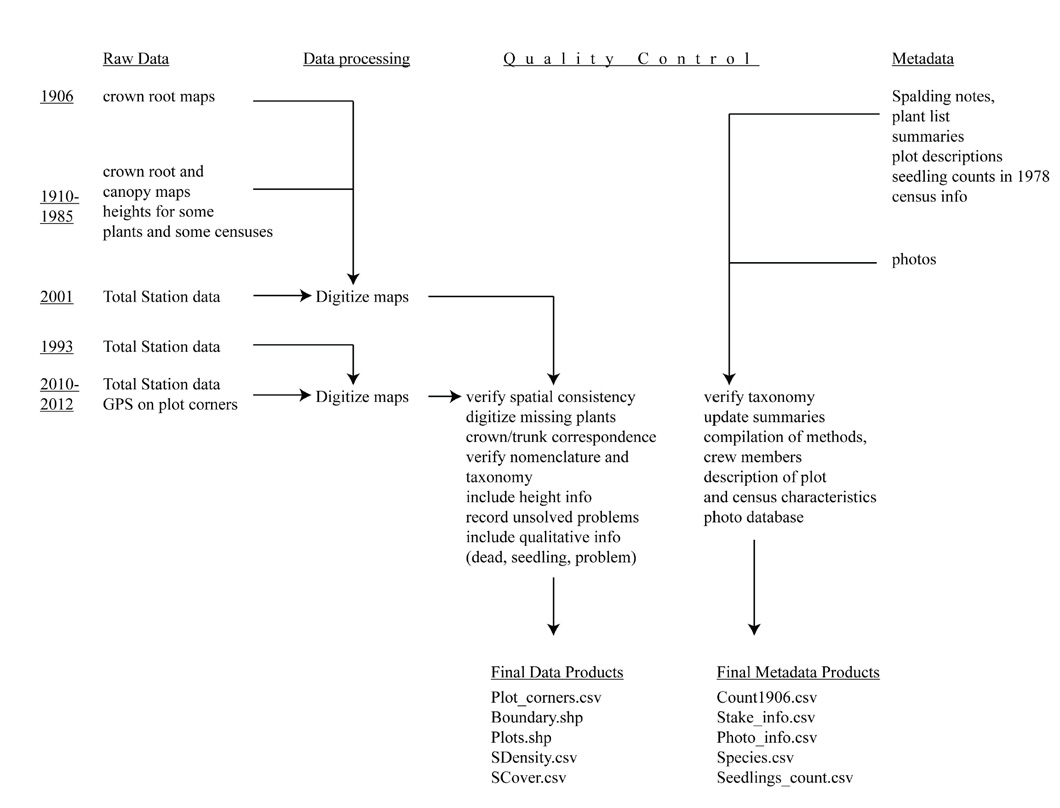
Fig. 3. Diagram depicting the overall procedures used during the archiving process.

Table 8 summarizes the plot census data sources used during this archiving effort. Only data prior to 2010 is included; see section II.B.3 for details on data for 2010–2012. Although most of the data was previously converted to digital forms in 2001 by SWCA, contracted by J. Bowers, during our archiving process we followed up this effort with a strict quality control on files generated in 2001. This effort also involved re-digitizing original data, and cross-referencing with original maps and plot summaries. For information on data forms and acquisition methods of repeat photography refer to sections III.B.1 and III.B.1

Table 8. Summary of procedures used during archiving process. Each row explains how data referenced in Table 7 was processed. Processing procedures complement information provided in section V.E.

2. Location of completed data forms:

Files derived from this project are located at the USGS in Tucson. See Table 7 for specific location of original maps, field notes, and additional information related to the Spalding-Shreve plots.

3. Data entry/verification procedures:

Verification of field data

There is no specific documentation of data verification for censuses between 1906 and 1959, although after every census, lead researchers generated plot summaries that cross-referenced information between the new and past censuses. During these procedures, several corrections were made and recorded on the original maps. These corrections usually involved nomenclature changes and correction on plant locations.

Between 1960 and 1985, R. M. Turner consistently verified field data using tallies of each species inside a 1 m x 1 m quadrant. With these tallies, R. M. Turner estimated gain and loses between two censuses for each quadrant. This procedure allowed detecting surviving and new plants as well as errors in plant nomenclature and plant locations. Turner also verified maps and plot summaries between 1906 and 1959 and generated quadrant-specific tallies for each census transition. In 1986, Turner and Goldberg also cross-referenced censuses to estimate individual plant histories and changes in individual plant canopy for every transition between 1906 and 1978. We used all this information to validate our digital version of the census maps.

Data from 2001 censuses were double-checked in the field by J. Bowers. At this point, canopies were smoothed with uncertain effect on the data, and species nomenclature was verified. Data from 1993 and 2010 censuses was verified during the archiving process (Section V.E). In particular, processing of field data from 2010–2012 started by generating polygons that represent plant canopies using ArcGIS 9.3. These polygons were later checked for inconsistencies in geometry. Some canopies were approximated using circles or rectangles from canopy dimensions taken during each census (see section II.B.3 for details). Final canopies were clipped to the 2001 or 2010 (only for plot 4) borders. Attribute tables were completed using attributes described in section IV.B.6 and data quality was verified as described in section V.E.1,

Verification of digitized data
For details on data verification see archiving Section V.E

B. Quality assurance/quality control procedures:

Field information

Plant identity, location, and cover

Between 1906 and 1985, field data was verified using quadrant-specific tallies (Section V.A.3). At the time of their censuses between 1910 and 1959, F. Shreve and A. Murray cross-referenced past censuses and made some corrections on the original maps. In particular, A. Murray made corrections in red on the 1936 and 1948 maps (Murray, unpublished field notes), and we have incorporated those corrections in the combined digital data.

Plant height

There is no information on quality assurance for height measurements taken between 1906 and 1985. The 1993 and 2010–2012 height data was double checked for abnormalities during data entry. No further verification has been conducted, and no further verification is likely.

Archiving process

See Section V.E

C. Related materials

See Table 7

D. Computer programs and data processing algorithms

For procedures used during archiving of data from 1906 to 2001 see archiving Section V.E.

E. Archiving

1. Archival procedures

Archiving of the Spalding-Shreve plot data has been conducted in two stages. In 2001, J. Bowers lead the first stage of the archiving process and conducted the 2001 census. At that time, Bowers compiled all available and pertinent information about the plots, and with the assistance of SWCA Environmental Consultants based in Tucson, they digitized original maps from 1906–1985 for plots 4, 7, 9–12, 14–16, and B1–B8. In 2010, S. Rodriguez-Buritica, with the assistance of H. Raichle and Bob Webb, started the second stage of the archiving process. This stage consisted of performing a rigorous quality control of outputs from 2001, completing the previous archives for data from lost plots (1–3, 5–6, 8, 17, 18) and secondary information regarding seedlings, annuals, and plant heights. In addition, during this second archiving effort, data from 1993 was rescued from computer printouts and integrated into the archives. The new censuses between 2010 and 2012 were integrated as well (Fig. 3). For specific procedures conducted during both stages of archiving please refer to Table 8.

Data verification during archiving

Procedures in 2001

In 2001, data verification consisted of cross-referencing plot tally sheets generated by R. M.Turner between 1960 and 1984 with similar summaries generated after digitization was finished. These tallies summarized density and cover changes between censuses without explicit identification of unique individuals. In addition, Bowers also used cover summaries per species to verify her cover summaries. With these procedures, in addition to cross-referencing maps from different years, she was able to detect and correct some errors, although there is no record of these corrections. Location of the final version of her maps as well as her density and cover summaries is given in Table 7. It is important to note that given the additional quality control procedures used during archiving in 2011, Bower’s information is not up-to-date and should not be used for ecological analyses in their original form.

Bowers et al. generated six shapefile types for each plot:

• Boundary: plot boundary derived from 2001 census with Total Station (TS)
• Control points: four plot corners for most plots, plus TS location taken during 2001 census
• Crowns and Rootsout: Outline of live canopies of plants rooted inside and outside a plot, respectively, after field census and smoothing
• Trunks and Points: Point location of root crowns of plants inside the plot with and without corresponding crown, respectively, after field census and ground proofing.

The only attribute recorded for each plant was the species name (following codes on file Species.csv), canopy area and perimeter.

Procedures in 2011–2012

We used the 2001 files as the starting point to generate a complete archive of all the ecological information associated with Spalding-Shreve plots; except the species enumerations on plot A (for this information see Bowers 1994, 2002, and Bowers et al. 2004) and the annual species list from 1983 (see Table 7 for location of these data). We focused on three tasks during this effort:

• Including information not considered during the 2001 archiving effort. This includes digitizing information related to lost plots (Fig. 1), secondary information on plant height and status at any census, seedling counts during 1978 census, and disturbance notes on any map. For a complete list of attributes see section IV.A. In addition to the secondary information recorded on maps, which was not included before, we also created a digital version of the original Spalding unpublished notes (file Count1906.csv). We cross-referenced the information from the notes with the original maps, recording any inconsistencies. We assumed map information was more reliable, and used this in subsequent comparisons across censuses. Inconsistencies usually correspond to mismatches in species number or identification.
• Including information on repeat photographs of the Spalding-Plots,
• Performing a rigorous quality control procedure on data digitized in 2001.

In the following section, we summarize the quality-control procedures. Problems that could not be solved during this quality control can be identified using the attribute tables associated with every shapefile (*.shp, see Tables 9 and 10 ).

Spatial consistency

Although Spalding and Shreve’s original intention was to delimit square plots of 10 m on a side, several, if not all, of the plots are not squares. As a consequence, maps generated by using a string grid and graph paper have a consistent error in the location and shape of plant features with respect to the real plot corners; this error was incorporated into the cover estimations reported before 2001. Using individual plant covers reported by Dodge in 1960 for plot 12, we estimated the difference between the two measurements (old map vs. corrected digital map) to be between -15.7 and 10.3 cm²  (n = 144, mean = -0.0270).

In addition to the errors generated from thinking the plots were perfect squares as described above, there were errors generated from the 2001 digitization process. Therefore our quality control process included checking and correcting the spatial consistency of all 2001 shapefiles. This verification was performed in ArcGIS 10 (ESRI) and included repairing any geometric problems. During GIS processing in 2001, paper maps were digitized and rectified to the plot corners surveyed with the Total Station (2001 control points.shp). Nevertheless, we identified major errors in this rectification; thus we used the following procedure to rectify any disagreement between the digital version of the maps and the original maps:

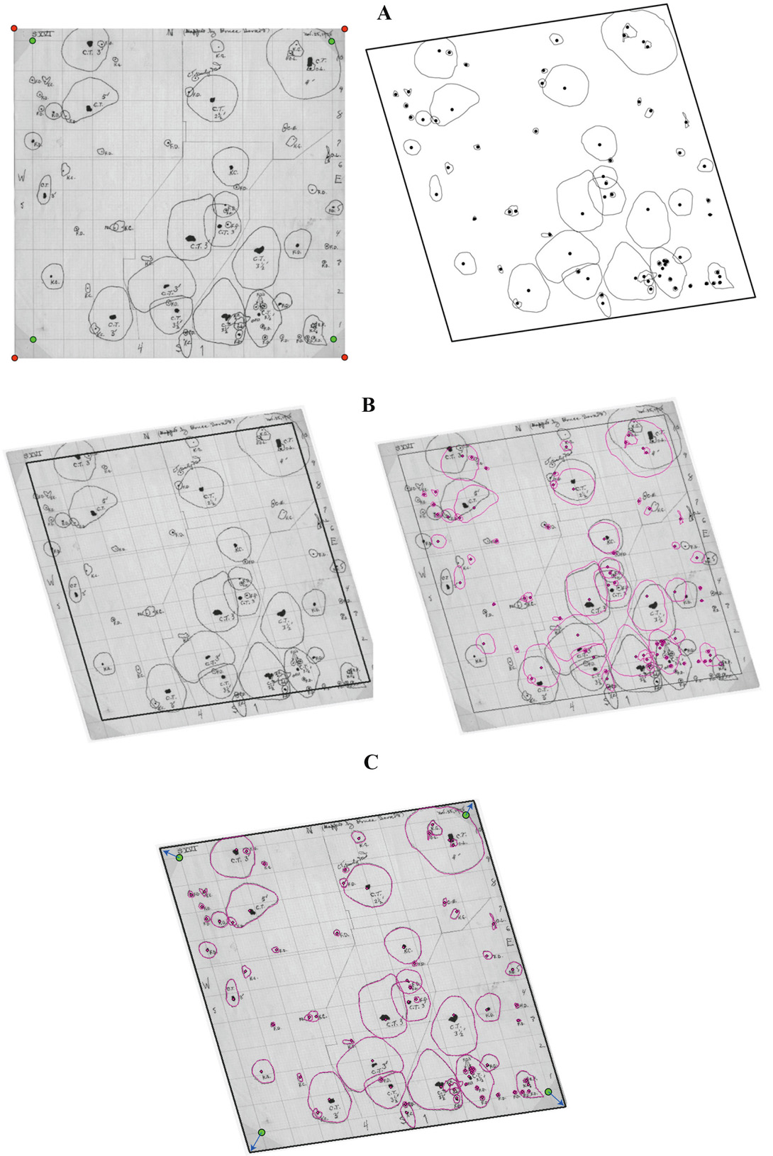
Fig. 4. Example of procedures used to check for spatial consistency among original and digitized maps using map of plot 16 in 1928.

1. We verified that the digital version of the maps from 2001 accurately capture the location of plant canopies with respect to the actual plot boundary. To do this, we scanned the original paper maps of the plots as *.tif files (Panel A, left in Fig 4) and then georeferenced the tifs (affine transformation) to the 2001 boundary shapefile using the plot corners as links (Panel B, left in Fig 4). Panel B, right shows  the 2001 digital version (Panel A, right) overlaid on our georeferenced tif (B, left).  

2. When plants did not align well after using the correct plot corners for georeferencing, we re-georeferenced the *.tif files linking the plant trunks , created control points on the correct plot corners (Panel C in Figure 4), and rubbersheeted all plant features to the corners of the boundary shapefile(using spatial adjustment/natural neighbor options in ArcGIS). This last procedure will expand or contract features within a digital map all at once By rubbersheeting the digital version  of the maps, we retained the overall spatial relation of all features on the maps while correcting the plot’s shape. For lost plots whose shape could not be verified with TS instrument, we used a 10 m x 10 m polygon to georeference the .tif files.

3. In cases where this previous steps did not produce satisfactory results and gross mismatches were still present between the original map and the digital version from 2001, we re-digitized the original paper maps (parts or the whole if necessary).

4. We clipped the final adjusted maps to the correct plot boundaries whenever necessary to produce the final corrected digital version of all paper maps.

In some instances (plots 4, 9, and 10), a large mismatch between 2001 and 2010–2012 plot boundaries evidenced errors in the identification of plot corners in the field. For plots 9 and 10 this mismatch was aggravated by the lack of permanent markers at plot corners. We estimated the correct location of corners using locations of large, persistent plants (Acacia, Cercidium, Larrea) relative to plot borders on maps prior to 2001. In the field, we used these distances to re-locate all plot corners, re-mapped their location, and adjusted all digital shapefiles to the resulting boundary. As a result of this adjustment, some areas within the plots were not censused in 2001 (nodata shapefile), which gives an underestimation of plant covers for plants close to these areas.

Missing shapes

In addition to checking for spatial consistency, we checked that all features on the original maps were included in the digital versions of the map. Previous analyses of these data and archiving in 2001 excluded species for which there had been an inconsistent enumeration (see Species.csv for a list of these species). In addition to including all species mapped, we checked that canopies of contiguous plots (Plots in area B) were accurately represented in all plots where they have canopy cover. In some censuses, some canopies were not complete, so we used a regular polygon (triangle or semicircle) to represent the missing canopies. The attributes associated with each shape allow identification of these non-original shapes. The only piece of information that we did not digitize corresponds to seedling mappings that were conducted after the overall plot census in the unusually wet year of 1978. Although we did not digitize this information, seedlings present during the summer of 1978 can be identified on the original map scans that we have provided.

Crown-trunk correspondence

Before and after spatial adjustments were made, we performed a spatial join of tables to check for correspondence between trunks and crowns. During this procedure, we identified several problems; these problems and our solutions are summarized in the tables 9–10.

Consistent identification of plants rooted in and outside the plots

We cross-referenced maps of different years to verify the consistent identification of plants in the plot boundaries (crowns) vs. outside (rootsout) each plot. We classified a plant as “in” or “out” of a plot based on the classification used over the majority of the censuses. Any change in the original assigment of a crown was recorded in the Attributes tables.

Species identity

We checked for consistent nomenclature using file Species.csv. In particular, we solved inconsistencies between root and canopy files, as well as misidentifications across census years.

Seedling identity

In general, there has been an inconsistent identifications of seedlings throughout censuses, and we used field notes and secondary information recorded on the maps to explicitly identify seedlings in our files; whenever possible.

Species-specific density and cover

Similar to Bowers in 2001, we used the density and cover summaries created by Turner to check for accurate enumeration and digitization of plants. Plants that were not previously counted are identified in the attribute tables. Using these procedures we identified and solved several errors in summaries generated by Goldberg and Turner (1986) and by Bowers in 2001. For this reason, our summary tables supersede all previous density and cover summaries.

Due to the uncertainty in field protocols at different censuses, there were several issues during the process of quality control that we could not solve. In this case, we recorded the pertinent information in the attribute table of the problematic record. Table 9 summarizes the problems we found when checking data from one map at the time, and Table 10 summarizes issues that arose when cross-referencing maps from different years.

Table 9. Problems when processing a single map. The following table summarizes problems detected during our quality-control procedures, and the solutions we used during archiving. Issues that could not be solved were recorded in the attribute tables of the *.shp files. For details of the columns used to record the problems, users should refer to section II.B.6

Table 10. Problems after cross-referencing. This table summarizes problems and solutions after cross-referencing censuses from different years or contiguous plots (plots in area B). Issues that could not be solved were recorded in the attribute tables of the *.shp files. For details of the columns used to record the problems refer to section II.B.6.

2. Redundant Archival sites

F. Publications and Results

The following is a list of publications that have directly used data from Spalding-Shreve plots:

Bowers, J. E. 1994. Natural conditions for seedling emergence of three woody species in the northern Sonoran Desert. Madroño 41:73–84.

Bowers, J. E. 2002. Regeneration of triangle-leaf bursage (Ambrosia deltoidea: Asteraceae): germination behaviour and persistent seed bank. Southwestern Naturalist 47:449–513.

Bowers, J. E. 2004. Temporal variation in longevity of Opuntia engelmannii (Cactaceae) flowers. Madroño 51:280–285.

Bowers, J. E., R. M. Turner, and T. L. Burgess. 2004. Temporal and spatial patterns in emergence and early survival of perennial plants at a Sonoran Desert site. Plant Ecology 172:107–119.

Bowers, J. E. 2005a. Effects of drought on shrub survival and longevity in the northern Sonoran Desert. Journal of the Torrey Botanical Society 132:421–431.

Bowers, J. E. 2005b. Influence of climatic variability on local population dynamics of a Sonoran Desert Platyopuntia. Journal of Arid Environments 61:193–210.

Bowers, J. E. 2010. A debt to the future: Achievements of the Desert Laboratory, Tumamoc Hill, Tucson, Arizona. Desert Plants 26:25–39.

Butterfield, B. J., J. L. Betancourt, R. Turner, and J. M. Briggs. 2010. Facilitation drives 65 years of vegetation change in the Sonoran Desert. Ecology 91: 1132–1139.

Goldberg, D. E., and R. M. Turner. 1986. Vegetation change and plant demography in permanent plots in the Sonoran Desert. Ecology 67:695–712.

Guo, Q. 2004. Slow recovery in Desert Perennial vegetation following Prolonged Human Disturbance. Journal of Vegetation Science 15:757–762.

Martin, S. C., and R. M. Turner. 1977. Vegetation change in the Sonoran Desert region: Arizona and Sonora. Journal of the Arizona Academy of Science 12:59–69.

Munson, S. M., R. H. Webb, J. Belnap, J. A. Hubbard, D. E. Swann, and S. Rutman. 2012. Forecasting climate change impacts to plant community composition in the Sonoran Desert region. Global Change Biology 18:1083–1095.

Murray, A. V. 1959. An analysis of changes in Sonoran Desert vegetation for the years 1928–1957. M.S. thesis, University of Arizona, Tucson, Arizona, USA.

Shreve, F. 1911. Establishment behavior of the palo verde. Plant World 14:289–299.

Shreve, F. 1917. The establishment of desert perennials. Journal of Ecology 5:210–216.

Shreve, F. 1929. Changes in desert vegetation. Ecology 10:364–373.

Shreve, F., and A. L. Hinckley. 1937. Thirty years of change in desert vegetation. Ecology 18:463–478.

Spalding, V. M. 1909. Distribution and Movements of Desert Plants. Publication No. 113, Carnegie Institution of Washington.

Webb, R. H., D. E. Boyer, and R. M. Turner. 2007. The Desert Laboratory Repeat Photography Collection—An invaluable archive documenting landscape change. U.S. Geological Survey Fact Sheet 2007-3046. http://pubs.usgs.gov/fs/2007/3046/.

Webb, R. H., and R. M. Turner. 2010. A debt to the Past: Long-term and current plant research at Tumamoc Hill in Tucson, Arizona. Desert Plants 26 (2):3–18.

G. History of data set usage

1.Data Request history

NA

2.Data set update history

3. Review History

NA

4. Questions and comments from secondary users

Maps used and arbitrary Cartesian coordinate system in meters. When maps are displayed using ArcGIS select “uknown” coordinate system and make sure “meters” is selected as preferred unit.

Acknowledgments

Special thanks is due the many colleagues that helped map the permanent plots in the last half century. These include R. A. Dodge, D. K. Warren, T. A. Gustafson, D. E. Goldberg, J. Conn, T. E. A. van Hylckama, L. H. Applegate, O. M. Grosz, Seth Munson, S. Carmichael, Margaret Snyder, and Diane Boyer. The authors thank J. Bowers for invaluable information she compiled; Michael List, Lara Mitchell, Roger Myers, S. Carmichael, and Diane Boyer for assistance during archiving process. We thank Seth Munson, and Alberto Burquez for critically reviewing this manuscript.

Literature cited

Bowers, J. E. 2005. Effects of drought on shrub survival and longevity in the northern Sonoran Desert. Journal of the Torrey Botanical Society 132:421–431.

Bowers, J. E. 2005. Influence of climatic variability on local population dynamics of a Sonoran Desert Platyopuntia. Journal of Arid Environments 61:193–210.

Bowers, J. E., and R. M. Turner. 1985. A revised vascular flora of Tumamoc Hill, Tucson, Arizona. Madroño 32:225–252.

Bowers, J. E. 2010. A debt to the future: Achievements of the Desert Laboratory, Tumamoc Hill, Tucson, Arizona. Desert Plants 26:25–39.

Butterfield, B. J., J. L. Betancourt, R. Turner, and J. M. Briggs. 2010. Facilitation drives 65 years of vegetation change in the Sonoran Desert. Ecology 91: 1132–1139.

Clements, F. E. 1916. Plant Succession: An Analysis of the Development of Vegetation. Washington D.C.: Carnegie Institution of Washington.

Goldberg, D. E., and R. M. Turner. 1986. Vegetation change and plant demography in permanent plots in the Sonoran Desert. Ecology 67:695–712.

Murray, A. V. 1959. An analysis of changes in Sonoran Desert vegetation for the years 1928-1957. M.S. thesis, University of Arizona, Tucson, Arizona, USA.

Shreve, F., and A.L. Hinckley. 1937. Thirty Years of Change in Desert Vegetation. Ecology 18:463–478.

The Taxonomic Name Resolution Service. 2012. Version 3.0 Published on the Internet: http://tnrs.iplantcollaborative.org (last accessed 26 November 2012).

Turner, R. M., R. H. Webb, J. E. Bowers, and J. R. Hastings. 2003. The Changing Mile Revisited. University of Arizona Press, Tucson, Arizona, USA.

USDA, NRCS. 2012. The PLANTS Database (http://plants.usda.gov, 17 January 2012). National Plant Data Team, Greensboro, NC 27401-4901 USA.

Wallace, H. D., P. R. Fish, and S. K. Fish. 2007. Tumamoc Hill and the early Pioneer Period occupation of the Tucson Basin. In S. K. Fish, P. R. Fish, and E. Villalpando, editors: Trincheras Sites in Time, Space, and Society., pp. 137–164. The University of Arizona Press, Tucson, Arizona, USA.

Webb, R. H., D. E. Boyer, and R. M. Turner, editors. 2010. Repeat Photography: Methods and Applications in the Natural Sciences. Island Press, Washington, D.C., USA.

Webb, R. H., D. E. Boyer, and R. M. Turner 2007. The Desert Laboratory Repeat Photography Collection—An invaluable archive documenting landscape change. U.S. Geological Survey Fact Sheet 2007-3046. http://pubs.usgs.gov/fs/2007/3046/

Webb, R. H., and R. M. Turner. 2010. A debt to the Past: Long-term and current plant research at Tumamoc Hill in Tucson, Arizona. Desert Plants 26(2):3–18.

[Back to E094-083]