Ecological Archives E095-149-D1

Elizabeth J. Sbrocco. 2014. Paleo-MARSPEC: gridded ocean climate layers for the mid-Holocene and Last Glacial Maximum. Ecology 95:1710. http://dx.doi.org/10.1890/14-0443.1

Metadata

Class I. Data set descriptors

A. Data set identity: Paleo-MARSPEC: Gridded ocean climate layers for the mid-Holocene and Last Glacial Maximum

B. Data set identification code: paleo-MARSPEC v1.1

C. Data set description

MARSPEC variables for the Last Glacial Maximum (LGM, approximately 21 ka) and mid-Holocene (MH, approximately 6 ka) derived from coupled ocean-atmosphere general circulation models submitted to the second phase of the Paleoclimate Modeling Intercomparison Project (PMIP2).

Principal Investigator: Elizabeth J. Sbrocco, National Evolutionary Synthesis Center, 2024 W. Main Street, Suite A200, Durham, NC 27705, USA, Email: [email protected]

Abstract: Understanding how species have responded to climate change during recent glacial cycles has the potential to inform our understanding of how species will respond to future climate change over the next century. Glacial refugia and historical range shifts over geological time have traditionally been inferred by examining the fossil record or the distributions of sister species using phylogeographic approaches and more recently, with species distribution models. Species distribution modeling has become a popular tool for projecting range expansions and contractions under climate-change scenarios in terrestrial ecosystems; however, such models are less commonly applied to the study of marine ecosystems despite a similar need for understanding species' vulnerabilities to fluctuating climates. Here I present gridded climatologies for the world ocean representing the annual mean, range, variance, and extremes in sea surface temperature and salinity for the mid-Holocene (6 ka) and the Last Glacial Maximum (LGM; 21 ka) obtained from coupled ocean–atmosphere general circulation models available through the second phase of the paleoclimate modeling intercomparison project (PMIP2). Furthermore, I present geophysical layers representing bathymetry, distance to shore, and six measures of topographic complexity during the LGM, when sea level was approximately 120 meters lower than today. All data layers are global in spatial extent, are downscaled to a 5-arc-minute spatial resolution, and are provided in ESRI raster grid format suitable for analysis in ArcGIS or in R using the raster package. These paleoclimatic data layers complement the modern bioclimatic and geophysical data layers contained in the MARSPEC database and should facilitate further studies on the historical response of marine species to late Quaternary climate change, including but not limited to inferences based on species distribution models.

D. Key words: ecological niche modeling; GIS; Last Glacial Maximum; late Quaternary climate; marine spatial ecology; mid-Holocene; ocean climate models; Pleistocene climate; species distribution modeling.

Class II. Research origin descriptors

A. Project description

Climatic fluctuations over the last two million years have had profound impacts on the distribution of species in both terrestrial and marine realms. As the Earth oscillated between glacial and interglacial periods during the Pleistocene, species responded by tracking spatial shifts in their preferred habitat, by adapting to novel climatic combinations, or by undergoing local or global extinction. Understanding the biological, geological, and climatic drivers of species responses to past global change is of academic interest to historical biogeographers but is also useful in a conservation context. This is because knowledge of what has driven a species' response to past climatic shifts can aid in the assessment of its extinction risk under future climate change scenarios, which in turn can be used to set conservation priorities. Gridded climate surfaces that can be manipulated in a GIS framework have been important tools for understanding species response to past climate change by allowing for spatially explicit hypotheses about range dynamics and community shifts to be tested against genetic and fossil evidence. The development of the global climate databases, such as WorldClim (Hijmans et al. 2005), which is based on long-term records of atmospheric temperature and precipitation, have facilitated these studies and have been used extensively for species distribution modeling (also called "ecological niche" or "bioclimatic envelope" modeling) in terrestrial systems. Furthermore, WorldClim variables based on past climates have also been useful for inferring range shifts over recent geological time and for identifying Pleistocene glacial refugia in terrestrial systems (e.g., Waltari et al. 2007; Carnaval and Moritz 2008; Svenning et al. 2011). 

Recently, global-scale ocean climate databases have been published for modeling marine species distributions under contemporary climate conditions (Tyberghein et al. 2012; Sbrocco and Barber 2013). The MARSPEC database (Sbrocco and Barber 2013) contains two types of data layers: geophysical variables that describe the bathymetry and topographic complexity of the ocean seafloor, and bioclimatic variables that summarize the annual mean, range, variance, and extremes in sea surface temperature and salinity based on in situ and remotely sensed climatic observations made during the late 20th and early 21st centuries (1955–2006 for salinity; 2002–2010 for temperature). The modern MARSPEC database also includes the long-term monthly averages ("climatologies") from which the summary bioclimatic variables were derived. These monthly climatologies allow for easy comparison of observed modern conditions to simulated climate of the past or future, since output from general circulation models (GCMs) is typically provided at a monthly temporal resolution for oceanic variables.

My goal here was to develop past climate analogues of the geophysical and bioclimatic variables contained within the MARSPEC ocean climate database in order to facilitate the study of marine species range dynamics in response to late Quaternary climate change. Reviews of differences between models and between models and proxy reconstructions are found elsewhere (e.g., Braconnot et al. 2007; Otto-Bliesner et al. 2009). For the bioclimatic layers, I focused on two climatic extremes over the last 21 thousand years (21 ka) that were simulated by coupled ocean-atmosphere general circulation models coordinated by the second phase of the Paleoclimate Modeling Intercomparison Project (PMIP2). The first climatic extreme is the Last Glacial Maximum (LGM), which occurred approximately 21 ka when glaciers were at their peak during the last ice age. The second climatic extreme occurred during the Mid-Holocene period (MH) approximately 6 ka when changes in Earth's orbit resulted in enhancement/reduction in the seasonal temperature cycle in the northern/southern hemisphere relative to modern seasonal cycles (Braconnot et al. 2007). The LGM data set is complemented by a new set of geophysical data layers based on a 120 meter drop in eustatic sea level due to the buildup of massive ice sheets on land (Fleming et al. 1998). The resulting "paleo-MARSPEC" database is provided for the world ocean in ESRI raster grid format that is easy to manipulate in ArcGIS (ESRI) or in R using the raster package (Hijmans 2013). It is also interpolated to a high spatial resolution of 5-arc-minutes, equal to approximately 9.2 km grid cell size at the equator. The spatial grid and extent are identical to the 5-arc-minute modern MARSPEC database, allowing for easy comparison between modern and past climatic periods. These grids are appropriate for use in marine paleo-species distribution models and other applications in marine spatial ecology.

B. Research methods

Bioclimatic Data

Simulated ocean climate data from the LGM and MH were obtained from coupled ocean–atmosphere general circulation models (OAGCMs) included in the PMIP2 database (Braconnot et al. 2007; http://pmip2.lsce.ipsl.fr). Only models that provided monthly data for both sea surface temperature (tos) and sea surface salinity (sos) were kept for analysis. Furthermore, the IPSL-CM4 model was excluded due to a corrupted file in the PMIP2 LGM output that had not been corrected by the time this manuscript was submitted.  Additionally, PMIP2 provides both MIROC 3.2 and MIROC 3.2.2 in the LGM database. These models are identical except that MIROC 3.2.2 corrects an error in the land surface scheme of the MIROC 3.2 model. Thus, the MIROC 3.2 model was excluded from the LGM data set, but kept in the Mid-Holocene dataset since MIROC 3.2.2 is not available for this time period. The resulting final dataset includes six models that simulate ocean climatic conditions during the LGM and eight models that simulate conditions during the MH (Table 1).

Table 1. PMIP2 models used to construct paleo-MARSPEC variables for the Mid-Holocene and Last Glacial Maximum. Averaging time is the number of model iterations (i.e., "model years") over which the mean monthly values were averaged to create the final variable. Grid spacing is irregular in most models, and so spatial resolution of the original model output is given as a global average. lon = longitude, lat = latitude, MH = Mid-Holocene Period, LGM = Last Glacial Maximum.

In order to create paleo-climate analogues of the modern bioclimatic MARSPEC variables, I obtained sea surface temperature and salinity data from PMIP2 models at a monthly temporal resolution. PMIP2 data were converted from NetCDF to xyz format using the reshape (Wickham 2007), ncdf (Pierce 2011), and fBasics (Wuertz et al. 2013) packages in R (scripts available at www.marspec.org). For each calendar month, I averaged over all model years available in the PMIP2 database, which varied by model (Table 1). OAGCMs are provided at coarse spatial resolutions and on irregular grids (Table 1), making them too coarse for regional to local-scale analyses and difficult to handle in GIS applications. Therefore, I downscaled the monthly climatologies to a 5-arc-minute regular spatial grid following the "delta" method (also called the "delta change" or "change factor" method) implemented by Ruegg et al. (2006) and Waltari et al. (2007).

There are many methods for downscaling climate data, and they range widely in complexity and underlying assumptions. The delta method is advantageous because it is simple, fast, and easy to implement across multiple models for the whole globe. The methods for downscaling can be broken into three main steps: calculation of temporal anomalies, interpolation, and calibration of modeled past climate data to modern observations. In Step 1, the temporal anomaly was calculated as the absolute difference between the mean monthly sea surface temperature or salinity value for the paleo-time period (the LGM or MH) and its baseline model (the "pre-industrial control", set around the year 1750). In the next step, the temporal anomalies were smoothed from the original model resolution to a 5-arc-minute spatial resolution via Inverse Distance Weighted (IDW) interpolation.  For the MH time slice, anomalies were interpolated within the same land/sea mask used for the modern MARSPEC database. For the LGM time slice, anomalies were interpolated within a land/sea mask altered by dropping sea level by 120 meters (see methods for geophysical data below). Finally, these interpolated anomalies were added to monthly climatologies for observed contemporary climate taken from the MARSPEC ocean climate database (Sbrocco and Barber 2013).

Bioclimatic variables that summarized the annual mean, range, variance, and extremes in sea surface temperature and salinity during the MH and LGM were calculated from these downscaled monthly data following the protocols of Sbrocco and Barber (2013). This resulted in the creation of 10 paleo-MARSPEC variables (Table 2) for which the modeled change in climate was calibrated to the modern observations captured by the original MARSPEC database. All variables were multiplied by a scaling factor to preserve precision (see Table 2) and converted to an integer in order to save on file space in the database.

Table 2. Definitions, units and scaling factors for geophysical and bioclimatic paleo-MARSPEC layers. Dividing variable by scaling factor converts the integer value to the unscaled floating point value. Note that the scaling factor for concavity differs here compared to the modern MARSPEC database. km = kilometers, psu = practical salinity units, °C = degrees Celsius.

Ensemble paleo-MARSPEC variables were also created from monthly climatologies averaged across all models for each time period. For the LGM experiment, only the CCSM3 model took into account a 1 psu (practical salinity unit) rise in ocean salinity due to the presence of large fresh-water ice sheets and drop in sea-level during the LGM (Shin et al. 2003; Braconnot et al. 2007). In order to place all models on the same scale for ensemble variable production, I followed DiNezio et al. (2011) and reduced salinity in the monthly climatologies for the CCSM3 model by 1 psu before calculating multi-model monthly ensemble means and subsequent paleo-MARSPEC variables (21kya__Ensemble_adjCCSM). This salinity adjustment was applied uniformly across the entire globe; however, it is possible that the change in salinity was regionally distributed (Braconnot et al. 2007), which would result in an over- or under-estimation of salinity in some geographic areas. Since this effect may be undesirable for some users, I also calculated an ensemble paleo-MARSPEC data set for the LGM that excludes CCSM3 (21kya__Ensemble_noCCSM). Users should note that the paleo-MARSPEC variables calculated from the CCSM3 model alone are based on the original model output and did not include the minus 1 psu salinity adjustment applied before ensemble calculation. The third phase of the Paleo-Modeling Intercomparison Project calls for all models to include the 1 psu salinity increase in LGM models, and so future updates of paleo-MARSPEC based on PMIP 3 output will incorporate this change in salinity.

Caveats and Assumptions Made in Creating Bioclimatic Variables

A limitation of working with the PMIP2 data set is that the control models used by this group were forced with pre-industrial (as opposed to present day) greenhouse gas concentrations. Pre-industrial conditions were used by the PMIP2 group because the Earth's climate system is not yet at equilibrium with recent increases in atmospheric greenhouse gases (Stouffer et al. 2004). In other words, even if greenhouse gases suddenly stopped increasing, atmospheric and oceanic temperatures would continue to rise for some time. Consequently, if the control models were run using present day greenhouse gas concentrations, they would simulate a modern climate that is too warm, yielding a past-modern climate anomaly that is too large. By using pre-industrial conditions, the PMIP2 pre-industrial control is on average slightly cooler than the observed present day conditions, yielding a past-modern climate anomaly that is too small. In the downscaling approach used here, calibrating the PMIP2 simulated climate to the MARSPEC observed modern climate using a temporal anomaly that is too small seems more conservative and less likely to produce serious errors than any other alternative. This approach is also widely used in the niche modeling literature to represent late Quaternary climate change from PMIP1 or PMIP2 model output relative to present day observed climate (e.g., Hijmans and Graham 2006, Ruegg 2006, Carstens and Richards 2007, Knowles et al. 2007, Waltari et al. 2007, Dépraz et al. 2008, Cordellier and Pfenninger 2009, Davies et al. 2009, and 55 others citing both the main PMIP2 paper [Braconnot et al. 2007] and the WorldClim database [Hijmans et al. 2005] used to downscale the paleoclimate data available at http://www.worldclim.org/downscaling). Efforts are currently underway by the third PMIP group to create present day and future climate models using the same model parameters as those used in paleo and pre-industrial models; thus, future versions of the paleo-MARSPEC database may not include this small-anomaly bias.

The delta method used to downscale the climate data makes the assumption that climate models produce reasonable estimates of the absolute difference (i.e., the anomaly) between the control run and past climate simulations, regardless of their skill in predicting the observed values during either time period (Hay et al 2000, Anandhi et al 2011). It also assumes that there is no spatial bias in the ability of the model to correctly estimate the anomaly between past and present conditions. These assumptions are not likely to be met in all locations or by all models, but can only truly be tested by comparing model data to proxy data (e.g., Otto-Bliesner et al. 2009, Hargreaves et al. 2011), the latter of which are scarce in many parts of the world. In the absence of widespread marine paleo-proxy records, inter-model variation may serve as an indicator of uncertainty in the data set and reveal spatial biases in how well the assumptions for downscaling via this method are met.

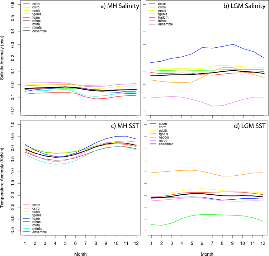
In order to visualize inter-model variation in the simulated sea surface temperature and salinity for each time period, I plotted anomaly data for each model by month (Fig. 1). MH simulations showed much better model agreement than LGM models, varying by less than 0.1 psu for salinity and by less than 0.5 Kelvin for temperature. On average, salinity was marginally more fresh during the MH and varied by less than 0.1 psu over the year. Temperature was, on average, about 0.25 Kelvin cooler during the MH boreal spring/austral fall than present and about 0.25 Kelvin warmer during the MH boreal fall/austral spring than present, while winter and summer were about the same as present. LGM simulations showed greater inter-model variation, varying on the order of 0.25–0.4 psu for salinity and by about 2 Kelvin for temperature, but for both variables this spread was due to only two of the six models. For LGM salinity, the HadCM3 model estimated the salinity anomaly to be approximately 0.1–0.15 psu greater than the ensemble model while the MIROC3.2.2 model estimated the salinity anomaly to be approximately 0.2 psu less than the ensemble model. The remaining four models differed from each other by less than 0.1 psu. Relative to modern times, sea surface salinity was estimated to be less than 0.1 psu saltier on average during the LGM, not taking into account the 1 psu salinity adjustment included in the original CCSM3 output. For LGM temperature, the CNRM model over-estimated the temperature anomaly by about 1 Kelvin relative to the ensemble while the FGOALS model under-estimated the ensemble temperature anomaly by about 1 Kelvin. The remaining models varied from each other by less than 0.5 Kelvin. On average, global sea surface temperature was estimated to be about 2 Kelvin cooler than present day during the LGM with little seasonal variance in the anomaly.

Fig. 1. PMIP2 model variation in simulating mean monthly salinity (A–B) and temperature (C–D) for the Mid-Holocene (A,C) and Last Glacial Maximum (B,D). CCSM in (B) is shown with a minus 1 psu salinity adjustment. Ensembles (black) are calculated as the average over all models.

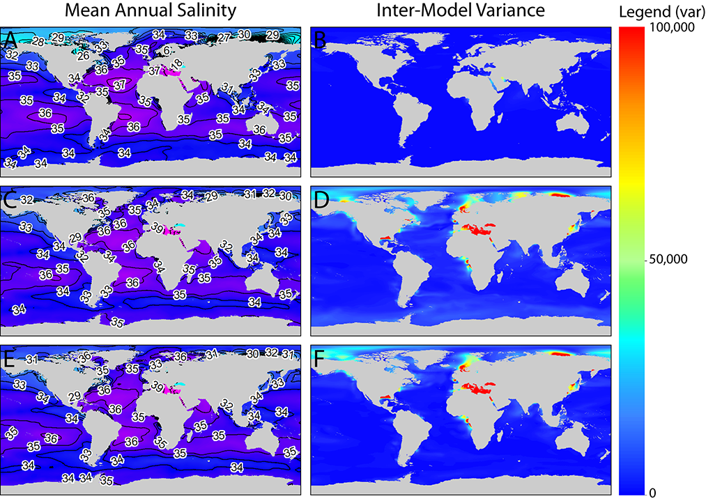
A map of ensemble annual means and the spatial distribution of inter-model variance for the MH and LGM are shown in Figs. 2–3. Figure 2b shows that inter-model variance for MH mean annual salinity is very low in most parts of the globe, with the exception of the Red Sea and Persian Gulf where inter-model variance is moderate. LGM mean annual salinity is higher (Fig. 2d,f), especially in areas with extremely high or low mean annual salinity. Inter-model variance in salinity was the highest in the Mediterranean Sea, the Black Sea, the Sea of Japan, the North Sea, the Arctic, and near the Mississippi and Congo Rivers.

Fig. 2. Paleo-MARSPEC ensemble mean annual sea surface salinity (biogeo08; left panel) and variance across individual models included in the ensemble (right panel) for the Mid-Holocene (A–B) and Last Glacial Maximum with (C–D) and without (E–F) the salinity-adjusted CCSM3 model. The figure legend applies to the Inter-Model Variance figures only (right panel). Lines in left panel are salinity contours measured in psu.

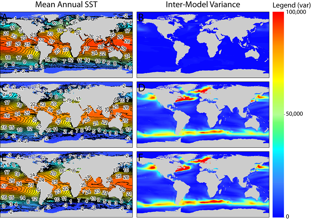
Inter-model variance for mean annual temperature showed different spatial patterns than salinity (Fig. 3). During the MH, inter-model variance was low across the entire globe (Fig. 3b); however, during the LGM (Fig. 3d,f), inter-model variance was high in temperate regions along the steep temperature gradients found in the western North Atlantic and western North Pacific, as well as subpolar regions along the Antarctic Convergence Zone and in the North Atlantic in the Barents and Norwegian Seas. For both salinity and temperature, spatial patterns of inter-model variance did not differ between ensemble models that included the CCSM3 model with the minus 1 psu salinity adjustment (Figs. 2c–d and 3c–d) and ensemble models that excluded the CCSM3 model (Figs. 2e–f and 3e–f).

Fig. 3. Paleo-MARSPEC ensemble mean annual sea surface temperature (biogeo13; left panel) and variance across individual models included in the ensemble (right panel) for the Mid-Holocene (A–B) and Last Glacial Maximum with (C–D) and without (E–F) the salinity-adjusted CCSM3 model. The figure legend applies to the Inter-Model Variance figures only (right panel). Lines in left panel are temperature contours measured in degrees Celsius.

An additional source of error lies in the IDW interpolation method used in downscaling the climate models. The major assumptions underlying IDW interpolation are that change in climate is spatially autocorrelated over a distance equal to or greater than the grain size of the original data set, and that the predicted value over the interpolated high-resolution grid is a linear function of distance from lower-resolution observations. IDW interpolation works best when point sampling is dense or when points are spaced along a regular grid, but the assumptions of IDW may be violated where the environmental gradient is steeper than the point density. In the PMIP2 models, points are spaced at gridded intervals that range from approximately 0.5–3.0 degrees latitude or longitude, depending on the model (see Table 1), and span the entire globe except for some coastal areas in the polar regions; therefore, IDW is expected to do a good job at smoothing the data across most of the globe. To test the skill of the interpolation method in reconstructing the original low resolution data, I calculated the root mean square error (RMSE) between the original data sets and the interpolated grids for the months of February and August for each model. RMSE ranged from 0.00004 to 0.01815, corresponding to R-squared values greater than 0.99 in all cases. This low error shows that the interpolated grid does an excellent job of representing the original data where data exists in the first place.

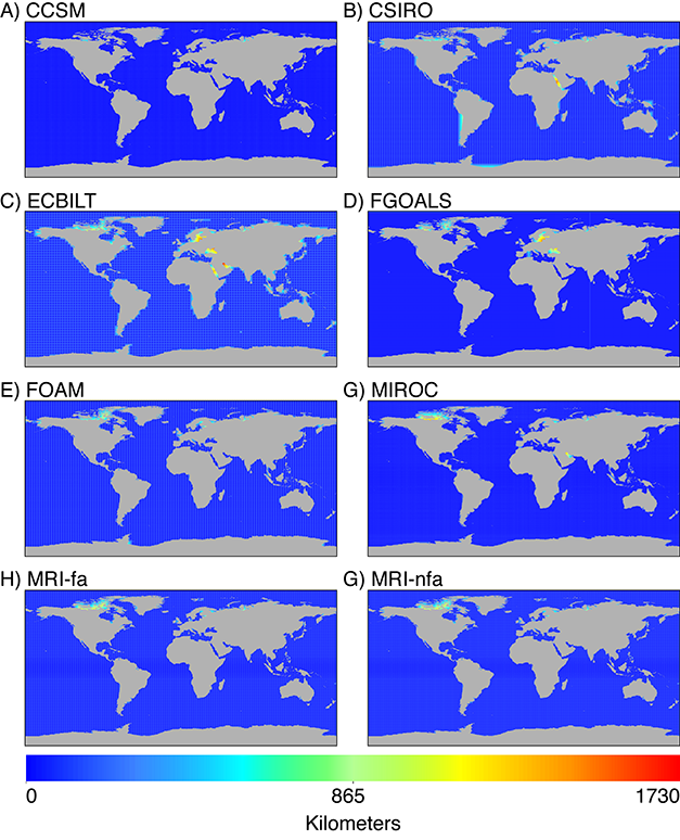
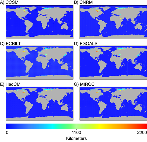
For each model, I also mapped the geographic distance between each high resolution pixel and its closest low resolution data point as an indicator of potential error from interpolation; greater error is expected where there is a greater distance to the nearest low resolution point. For the MH (Fig. 4), all models show decreased coverage in the Arctic Ocean north of North America. Several marginal seas were also unrepresented by the data in some models, indicating that not all models may be appropriate for small scale studies in these study systems. Both the CSIRO and ECBILT models show a large distance to the nearest low resolution point in the Red Sea. Furthermore, ECBILT and FGOALS lack points in the Baltic and Black Seas, and ECBILT and MIROC lack points in the Persian Gulf. Some marginal seas were similarly under-represented by model data during the LGM for some models. All models lacked data in the Barents and Kara Seas north of Russia and in the Hudson Bay. Furthermore, the CNRM, ECBILT, and FGOALS models lacked data in the Black Sea and Red Sea. The FGOALS model also lacked data in the Sea of Japan. All other areas were well represented by model data.

Fig. 4. Distance to nearest low-resolution point used in IDW interpolation for all PMIP2 models of the Mid-Holocene time slice.

Fig. 5. Distance to nearest low-resolution point used in IDW interpolation for all PMIP2 models of the LGM time slice.

Geophysical Data

To model the eustatic drop in sea level due to the buildup of ice sheets on land during the LGM, I added 120 meters to the modern MARSPEC 5-arc-minute bathymetry grid and changed values above or equal to 0 to NO DATA. Aspect (N/S and E/W), curvature (plan and profile), slope, concavity, and distance to shore were calculated from this new bathymetry grid following the protocols of Sbrocco and Barber (2013) for geophysical variables (biogeo01-07; Table 2). All variables were multiplied by a scaling factor (see Table 2) and converted to an integer in order to save on file space in the database. These scaling factors were identical to those used in the modern MARSPEC database with the exception of concavity, which was multiplied by 10,000 in the LGM database instead of 1,000 as in the modern database. The boundary conditions for the PMIP2 models call for the use of modern topography and coastline in MH models (see PMIP2 boundary conditions: http://pmip2.lsce.ipsl.fr); therefore, no new geophysical layers are provided for use with the MH bioclimatic paleo-MARSPEC variables. Instead, users can obtain bathymetry and measures of topographic complexity (biogeo01-07) from the 5-arc-minute modern MARSPEC database (Sbrocco and Barber 2013), which uses the same land-mask as the MH bioclimatic variables.

Class III. Data set status and accessibility

A. Status

Latest update: October 2013.

B. Accessibility

Storage location and medium: The Ecological Society of America provides long-term storage for these data through their Ecological Archives. Data can be downloaded directly from the data archive. The principal investigator also maintains a digital copy of the full data set. Links to the ESA data archive and a summary of the available data files can be found on the project website, http://www.marspec.org.

Contact person: Elizabeth J. Sbrocco, National Evolutionary Synthesis Center, 2024 W. Main Street, Suite A200, Durham, NC 27705, USA, E-mail: [email protected]

Copyright restrictions: None.

Proprietary restrictions: Users should cite this publication and Braconnot et al. (2007). The original data sets from which these climate layers were derived can be obtained from the PMIP2 project website (http://pmip2.lsce.ipsl.fr/).

Costs: None.

Class IV. Data structural descriptors

A. Data Set File

Identity: 6kya__Ensemble.7z

Size: 36,753,661 bytes

Format and storage mode: ESRI raster grids at 5-arc-minute spatial resolution (approximately 9.2 km grid cell sizes at the equator) for bioclimatic paleo-MARSPEC variables derived from the Mid-Holocene ensemble model averaged over the CCSM3, CSIRO, ECBILTCLIOVECODE, FGOALS, FOAM, MIROC3.2, MRI-fa, and MRI-nfa mid-Holocene PMIP2 models. Ten grids are compressed together in a single 7-zip archive. 7-zip archives can be unpacked with various zip utility programs, including 7-Zip 9.20 (open-source, http://www.7-zip.org/) and WinZip (proprietary, http://www.winzip.com). All ESRI grids are unprojected in the WGS84 Geographic Coordinate System.

A2. Data set file

Identity: 6kya_CCSM.7z

Size: 37,800,263 bytes

Format and storage mode: ESRI raster grids at 5-arc-minute spatial resolution (approximately 9.2 km grid cell sizes at the equator) for bioclimatic paleo-MARSPEC variables derived from the PMIP2 Mid-Holocene CCSM3 model. Ten grids are compressed together in a single 7-zip archive. 7-zip archives can be unpacked with various zip utility programs, including 7-Zip 9.20 (open-source, http://www.7-zip.org/) and WinZip (proprietary, http://www.winzip.com). All ESRI grids are unprojected in the WGS84 Geographic Coordinate System.

A3. Data set file

Identity: 6kya_CSIRO.7z

Size: 37,238,558 bytes

Format and storage mode: ESRI raster grids at 5-arc-minute spatial resolution (approximately 9.2 km grid cell sizes at the equator) for bioclimatic paleo-MARSPEC variables derived from the PMIP2 mid-Holocene CSIRO model. Ten grids are compressed together in a single 7-zip archive. 7-zip archives can be unpacked with various zip utility programs, including 7-Zip 9.20 (open-source, http://www.7-zip.org/) and WinZip (proprietary, http://www.winzip.com). All ESRI grids are unprojected in the WGS84 Geographic Coordinate System.

A4. Data set file

Identity: 6kya_ECBILTCLIOVECODE.7z

Size: 36,705,584 bytes

Format and storage mode: ESRI raster grids at 5-arc-minute spatial resolution (approximately 9.2 km grid cell sizes at the equator) for bioclimatic paleo-MARSPEC variables derived from the PMIP2 Mid-Holocene ECBILTCLIOVECODE model. Ten grids are compressed together in a single 7-zip archive. 7-zip archives can be unpacked with various zip utility programs, including 7-Zip 9.20 (open-source, http://www.7-zip.org/) and WinZip (proprietary, http://www.winzip.com). All ESRI grids are unprojected in the WGS84 Geographic Coordinate System.

A5. Data set file

Identity: 6kya_FGOALS.7z

Size: 36,790,529 bytes

Format and storage mode: ESRI raster grids at 5-arc-minute spatial resolution (approximately 9.2 km grid cell sizes at the equator) for bioclimatic paleo-MARSPEC variables derived from the PMIP2 mid-Holocene FGOALS model. Ten grids are compressed together in a single 7-zip archive. 7-zip archives can be unpacked with various zip utility programs, including 7-Zip 9.20 (open-source, http://www.7-zip.org/) and WinZip (proprietary, http://www.winzip.com). All ESRI grids are unprojected in the WGS84 Geographic Coordinate System.

A6. Data set file

Identity: 6kya_FOAM.7z

Size: 37,193,621 bytes

Format and storage mode: ESRI raster grids at 5-arc-minute spatial resolution (approximately 9.2 km grid cell sizes at the equator) for bioclimatic paleo-MARSPEC variables derived from the PMIP2 Mid-Holocene FOAM model. Ten grids are compressed together in a single 7-zip archive. 7-zip archives can be unpacked with various zip utility programs, including 7-Zip 9.20 (open-source, http://www.7-zip.org/) and WinZip (proprietary, http://www.winzip.com). All ESRI grids are unprojected in the WGS84 Geographic Coordinate System.

A7. Data set file

Identity: 6kya_MIROC-32.7z

Size: 37,776,932 bytes

Format and storage mode: ESRI raster grids at 5-arc-minute spatial resolution (approximately 9.2 km grid cell sizes at the equator) for bioclimatic paleo-MARSPEC variables derived from the PMIP2 Mid-Holocene MIROC 3.2 model. Ten grids are compressed together in a single 7-zip archive. 7-zip archives can be unpacked with various zip utility programs, including 7-Zip 9.20 (open-source, http://www.7-zip.org/) and WinZip (proprietary, http://www.winzip.com). All ESRI grids are unprojected in the WGS84 Geographic Coordinate System.

A8. Data set file

Identity: 6kya_MRI-fa.7z

Size: 37,624,110 bytes

Format and storage mode: ESRI raster grids at 5-arc-minute spatial resolution (approximately 9.2 km grid cell sizes at the equator) for bioclimatic paleo-MARSPEC variables derived from the PMIP2 mid-Holocene MRI-fa model. Ten grids are compressed together in a single 7-zip archive. 7-zip archives can be unpacked with various zip utility programs, including 7-Zip 9.20 (open-source, http://www.7-zip.org/) and WinZip (proprietary, http://www.winzip.com). All ESRI grids are unprojected in the WGS84 Geographic Coordinate System.

A9. Data set file

Identity: 6kya_MRI-nfa.7z

Size: 37,395,704 bytes

Format and storage mode: ESRI raster grids at 5-arc-minute spatial resolution (approximately 9.2 km grid cell sizes at the equator) for bioclimatic paleo-MARSPEC variables derived from the PMIP2 mid-Holocene MRI-nfa model. Ten grids are compressed together in a single 7-zip archive. 7-zip archives can be unpacked with various zip utility programs, including 7-Zip 9.20 (open-source, http://www.7-zip.org/) and WinZip (proprietary, http://www.winzip.com). All ESRI grids are unprojected in the WGS84 Geographic Coordinate System.

A10. Data set file

Identity: 21kya__Ensemble_adjCCSM.7z

Size: 35,091,931 bytes

Format and storage mode: ESRI raster grids at 5-arc-minute spatial resolution (approximately 9.2 km grid cell sizes at the equator) for bioclimatic paleo-MARSPEC variables derived from the PMIP2 LGM ensemble model averaged over the CCSM3 LGM model with a minus 1 psu salinity adjustment and the CNRM, ECBILTCLIO, FGOALS, HadCM, and MIROC 3.2.2 LGM PMIP2 models. Ten grids are compressed together in a single 7-zip archive. 7-zip archives can be unpacked with various zip utility programs, including 7-Zip 9.20 (open-source, http://www.7-zip.org/) and WinZip (proprietary, http://www.winzip.com). All ESRI grids are unprojected in the WGS84 Geographic Coordinate System.

A11. Data set file

Identity: 21kya__Ensemble_noCCSM.7z

Size: 35,207,860 bytes

Format and storage mode: ESRI raster grids at 5-arc-minute spatial resolution (approximately 9.2 km grid cell sizes at the equator) for bioclimatic paleo-MARSPEC variables derived from the PMIP2 LGM ensemble model averaged over the CNRM, ECBILTCLIO, FGOALS, HadCM, and MIROC 3.2.2 LGM PMIP2 models. This ensemble excludes the CCSM3 model. Ten grids are compressed together in a single 7-zip archive. 7-zip archives can be unpacked with various zip utility programs, including 7-Zip 9.20 (open-source, http://www.7-zip.org/) and WinZip (proprietary, http://www.winzip.com). All ESRI grids are unprojected in the WGS84 Geographic Coordinate System.

A12. Data set file

Identity: 21kya_CCSM.7z

Size: 37,178,848 bytes

Format and storage mode: ESRI raster grids at 5-arc-minute spatial resolution (approximately 9.2 km grid cell sizes at the equator) for bioclimatic paleo-MARSPEC variables derived from the PMIP2 LGM CCSM3 model. No salinity adjustments were made to the original data from the PMIP2 database for these variables. In other words, this model includes a 1 psu salinity increase relative to other LGM salinity models included in this package. Ten grids are compressed together in a single 7-zip archive. 7-zip archives can be unpacked with various zip utility programs, including 7-Zip 9.20 (open-source, http://www.7-zip.org/) and WinZip (proprietary, http://www.winzip.com). All ESRI grids are unprojected in the WGS84 Geographic Coordinate System.

A13. Data set file

Identity: 21kya_CNRM.7z

Size: 35,193,172bytes

Format and storage mode: ESRI raster grids at 5-arc-minute spatial resolution (approximately 9.2 km grid cell sizes at the equator) for bioclimatic paleo-MARSPEC variables derived from the PMIP2 LGM CNRM model. Ten grids are compressed together in a single 7-zip archive. 7-zip archives can be unpacked with various zip utility programs, including 7-Zip 9.20 (open-source, http://www.7-zip.org/) and WinZip (proprietary, http://www.winzip.com). All ESRI grids are unprojected in the WGS84 Geographic Coordinate System.

A14. Data set file

Identity: 21kya_ECBILTCLIO.7z

Size: 34,912,659 bytes

Format and storage mode: ESRI raster grids at 5-arc-minute spatial resolution (approximately 9.2 km grid cell sizes at the equator) for bioclimatic paleo-MARSPEC variables derived from the PMIP2 LGM ECBILTCLIO model. Ten grids are compressed together in a single 7-zip archive. 7-zip archives can be unpacked with various zip utility programs, including 7-Zip 9.20 (open-source, http://www.7-zip.org/) and WinZip (proprietary, http://www.winzip.com). All ESRI grids are unprojected in the WGS84 Geographic Coordinate System.

A15. Data set file

Identity: 21kya_FGOALS.7z

Size: 34,921,648 bytes

Format and storage mode: ESRI raster grids at 5-arc-minute spatial resolution (approximately 9.2 km grid cell sizes at the equator) for bioclimatic paleo-MARSPEC variables derived from the PMIP2 LGM FGOALS model. Ten grids are compressed together in a single 7-zip archive. 7-zip archives can be unpacked with various zip utility programs, including 7-Zip 9.20 (open-source, http://www.7-zip.org/) and WinZip (proprietary, http://www.winzip.com). All ESRI grids are unprojected in the WGS84 Geographic Coordinate System.

A16. Data set file

Identity: 21kya_HadCM.7z

Size: 39,329,926 bytes

Format and storage mode: ESRI raster grids at 5-arc-minute spatial resolution (approximately 9.2 km grid cell sizes at the equator) for bioclimatic paleo-MARSPEC variables derived from the PMIP2 LGM HadCM model. Ten grids are compressed together in a single 7-zip archive. 7-zip archives can be unpacked with various zip utility programs, including 7-Zip 9.20 (open-source, http://www.7-zip.org/) and WinZip (proprietary, http://www.winzip.com). All ESRI grids are unprojected in the WGS84 Geographic Coordinate System.

A17. Data set file

Identity: 21kya_MIROC-322.7z

Size: 36,755,950 bytes

Format and storage mode: ESRI raster grids at 5-arc-minute spatial resolution (approximately 9.2 km grid cell sizes at the equator) for bioclimatic paleo-MARSPEC variables derived from the PMIP2 LGM MIROC 3.2.2 model. Ten grids are compressed together in a single 7-zip archive. 7-zip archives can be unpacked with various zip utility programs, including 7-Zip 9.20 (open-source, http://www.7-zip.org/) and WinZip (proprietary, http://www.winzip.com). All ESRI grids are unprojected in the WGS84 Geographic Coordinate System.

A18. Data set file

Identity: 21kya_Geophysical_Data.7z

Size:; 30,403,463 bytes

Format and storage mode: ESRI raster grids at 5-arc-minute spatial resolution (approximately 9.2 km grid cell sizes at the equator) for bathymetry and geophysical paleo-MARSPEC variables derived to accompany the LGM bioclimatic paleo-MARSPEC variables. Eight grids are compressed together in a single 7-zip archive. 7-zip archives can be unpacked with various zip utility programs, including 7-Zip 9.20 (open-source, http://www.7-zip.org/) and WinZip (proprietary, http://www.winzip.com). All ESRI grids are unprojected in the WGS84 Geographic Coordinate System.

Class V. Supplemental descriptors

A. Data acquisition

Data can be downloaded directly from ESA's Ecological Archives or indirectly through the author's project website: http://www.marspec.org.

B. Related materials:

The paleo-MARSPEC data published here are meant to complement the geophysical and bioclimatic MARSPEC variables for contemporary climate that are published in the ESA's Ecological Archives (Sbrocco and Barber 2013; http://dx.doi.org/10.1890/12-1358.1).

C. Computer programs and data-processing algorithms

R-scripts for converting PMIP2 netCDF files to XYZ format and ArcGIS 10.0 ModelBuilder flowchart of GIS processing steps are available through the author's project website: http://www.marspec.org.

D. Publications and results

The author has several articles in prep that use this data set.

Acknowledgments

I acknowledge the international modeling groups for providing their data for analysis and the Laboratoire des Sciences du Climat et de l'Environnement (LSCE) for collecting and archiving the model data. The PMIP2 Data Archive is supported by CEA, CNRS, and the Programme National d'Etude de la Dynamique du Climat (PNEDC). The analyses were performed using version 01-21-2010 of the database. More information is available on http://pmip2.lsce.ipsl.fr/. This material is based upon work supported by the National Science Foundation through the National Evolutionary Synthesis Center (NESCent) under grant number NSF #EF-0905606.

Literature cited

Anandhi, A., A. Frei, D. C. Pierson, E. M. Schneiderman, M. S. Zion, D. Lounsbury, and A. H. Matonse. 2011. Examination of change factor methodologies for climate change impact assessment. Water Resources Research, 47, W03501, doi:10.1029/2010WR009104.

Braconnot P., B. Otto-Bliesner, S. Harrison, S. Joussaume, J.-Y. Peterschmitt, A. Abe-Ouchi, M. Crucifix, E. Driesschaert, Th. Fichefet, C. D. Hewitt, M. Kageyama, A. Kitoh, A. Laîné, M.-F. Loutre, O. Marti, U. Merkel, G. Ramstein, P. Valdes, S. L.Weber, Y. Yu, and Y. Zhao. 2007. Results of PMIP2 coupled simulations of the Mid-Holocene and Last Glacial Maximum - Part 1: experiments and large-scale features. Climate of the Past 3(2):261–277.

Carnaval, A. C., and C. Moritz. 2008. Historical climate modelling predicts patterns of current biodiversity in the Brazilian Atlantic forest. Journal of Biogeography 35:1187–1201.

Carstens, B. C., and C. L. Richards. 2007. Integrating coalescent and ecological niche modeling in comparative phylogeography. Evolution 61:1439–1454.

Cordellier, M., and M. Pfenninger. 2009. Inferring the past to predict the future: phylogeography and climate modelling predictions for the freshwater gastropod Radix balthica (Pulmonata, Basommatophora). Molecular Ecology 18:534–544.

Davies T. J., A. Purvis, and J. L. Gittleman. 2009. Quaternary climate change and the geographic ranges of mammals. American Naturalist 174:297–307.

Dépraz A., J. Cordellier, J. Hausser and H. Pfenninger. 2008. Postglacial recolonization at a snail's pace (Trochulus villosus): confronting competing refugia hypotheses using model selection. Molecular Ecology 17:2449–2462.

DiNezio, P. N., A. Clement, G. A. Vecchi, B. Soden, A. J. Broccoli, B. L. Otto-Bliesner, and P. Braconnot. 2011. The response of the Walker circulation to the Last Glacial Maximum forcing: Implications for detection in proxies. Paleoceanography 26, PA3217, doi: 10.1029/2010PA002083.

Fleming K., P. Johnston, D. Zwartz, Y. Yokoyama, K. Lambeck, and J. Campbell. 1998. Refining the eustatic sea-level curve since the Last Glacial Maximum using far- and intermediate-field sites. Earth and Planetary Science Letters 163:327–342.

Hargreaves J. C., A. Paul, R. Ohgaito, A. Abe-Ouchi and J.D. Annan. 2011. Are paleoclimate model ensembles consistent with the MARGO data synthesis? Climate of the Past 7: 917–933.

Hay, L. E., R. L. Wilby, and G. H. Leavesley. 2000. A comparison of delta change and downscaled GCM scenarios for three mountainous basins in the United States. Journal of the American Water Resources Association 36(2):387–397.

Hijmans R. J., S. E. Cameron, J. L. Parra, P. G. Jones, and A. Jarvis. 2005. Very high resolution interpolated climate surfaces for global land areas. International Journal of Climatology 25:1965–1978.

Hijmans, R. J., and C. H. Graham. 2006. The ability of climate envelope models to predict the effect of climate change on species distributions. Global Change Biology 12:1–10.

Hijmans, R. J. 2013. raster: raster: Geographic data analysis and modeling. R package version 2.1-49. http://CRAN.R-project.org/package=raster

Knowles, L. L., B. C. Carstens, and M. L. Keat. 2007. Coupling genetic and ecological-niche models to examine how past population distributions contribute to divergence. Current Biology 17:940–946.

Otto-Bliesner, B. L., R. Schneider, E. C. Brady, M. Kucera, A. Abe-Ouchi, E. Bard, P. Braconnot, M. Crucifix, C. D. Hewitt, M. Kageyama, O. Marti, A. Paul, A. Rosell-Melé, C. Waelbroeck, S. L. Weber, M. Weinelt and Y. Yu. 2009. A comparison of PMIP2 model simulations and the MARGO proxy reconstruction for tropical sea surface temperatures at last glacial maximum. Climate Dynamics 32:799–815.

Pierce D. 2011. ncdf: Interface to Unidata netCDF data files. R package version 1.6.6. http://CRAN.R-project.org/package=ncdf.

Ruegg, K. C., R. J. Hijmans, and C. Moritz. 2006. Climate change and the origin of migratory pathways in the Swainson's thrush, Catharus ustulatus. Journal of Biogeography 33:1172–1182.

Sbrocco, E. J., and P. H. Barber. 2013. MARSPEC: Ocean climate layers for marine spatial ecology. Ecology 94:979.

Shin S.-I., Z. Liu, B. Otto-Bliesner, E. C. Brady, J. E. Kutzbach, and S. P. Harrison. 2003. A simulation of the Last Glacial Maximum using the NCAR-CCSM. Climate Dynamics 20:127–151.

Svenning, J. C., C. Fløjgaard, K. A. Marske, D. Nógues-Bravo, and S. Normand. 2011. Applications of species distribution modeling to paleobiology. Quaternary Science Reviews 30:2930–2947.

Tyberghein, L., H. Verbruggen, K. Pauly, C. Troupin, F. Mineur, and O. De Clerck. 2012. Bio-ORACLE: a global environmental dataset for marine species distribution modelling. Global Ecology and Biogeography 21:272–281.

Waltari E., R. J. Hijmans, A. T. Peterson, A. S. Nyári, S. L. Perkins, and R. P. Guralnick. 2007. Locating pleistocene refugia: Comparing phylogeographic and ecological niche model predictions. PLoS ONE 2:e563.

Wickham, H. 2007. Reshaping data with the reshape package. Journal of Statistical Software 21(12).

Wuertz, D., and Rmetrics core team members. 2013. fBasics: Rmetrics - Markets and Basic Statistics. R package version 3010.86. http://CRAN.R-project.org/package=fBasics

[Back to E095-149]